"main directions" followed by the molecule's 3N degrees of freedom, or, in other words, the
directions followed collectively by the atoms. Interpolating along each PC makes each atom
follow a linear trajectory, that corresponds to the direction of motion that explains the most data
variance. For this reason, the PCs are often called Main Modes of Motion or Collective Modes of
Motion when computed from molecular motion data. Interpolating along the first few PCs has the
effect of removing atomic "vibrations" that are normally irrelevant for the molecule's bigger scale
motions, since the vibration directions have little data variance and would correspond to the last
(least important) modes of motion. It is now possible to define a lower-dimensional subspace of
protein motion spanned by the first few principal components and to use these to project the initial
high-dimensional data onto this subspace. Since the PCs are displacements (and not positions), in
order to interpolate conformations along the main modes of motion one has to start from one of
the known structures and add a multiple of the PCs as perturbations. In mathematical terms, in
order to produce conformations interpolated along the first PC one can compute:
Where c is a molecular conformation from the (aligned) data set and the interpolating parameter
can be used to add a deviation from the structure c along the main direction of motion. The
parameter can be either positive or negative. However, it is important to keep in mind that large
values of the interpolating parameter will start stretching the molecule beyond physically
acceptable shapes, since the PCs make all atoms follow straight lines and will fairly quickly
destroy the molecule's topology. A typical way of improving the physical feasibility of
interpolated conformations is to subject them to a few iterations of energy minimization following
some empirical force field.
Although it is possible to determine as many principal components as the number of original
variables (3N), PCA is typically used to determine the smallest number of uncorrelated principal
components that explain a large percentage of the total variation in the data, as quantified by the
residual variance. The exact number of principal components chosen is application-dependent and
constitutes a truncated basis of representation.
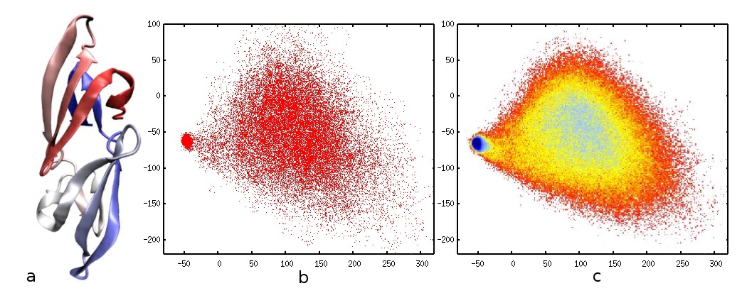
As an example of the application of PCA to produce low-dimensional points for high-dimensional
input, consider the Cyanovirin-N (CV-N) protein depicted in figure 4 a), corresponding to PDB
code 2EZM. This protein acts as a virucidal for many viruses, such as HIV. Protein folding
simulations of this protein can be used as input for a PCA analysis. A model of this protein that
considers atoms at the alpha-carbon positions only has 101 such atoms, for a total of 303 degrees
of freedom. Folding/unfolding simulations starting from the native PDB structure produce
abundant conformation samples of CV-N along the folding reaction.
Figure 72.
CV-N protein and PCA projections. a) A cartoon rendering of the CV-N protein. b) The projection of each simulated conformation onto the first two PCs. The concentrated cluster to the left corresponds to the "folded" protein, and the more spread cluster to the right corresponds to the "unfolded" protein. c) The PCA coordinates used as a basis for a free-energy (probability) plot.
Figure 4 b) shows the projection of each simulated conformation onto the first two principal
components. Each point in the plot corresponds to exactly one of the input conformations, which
have been classified along the first two PCs. Note that even the first PC alone can be used to
approximately classify a conformation as being "folded" or "unfolded", and the second PC
explains more of the data variability by assigning a wider spread to the unfolded region (for which
the coordinate variability is much larger). The low-dimensional projections can be used as a basis
to compute probability and free-energy plots, for example as in Das et al. [link] Figure 4 c) shows such a plot for CV-N, which makes the identification of clusters easier. Using PCA to interpolate
conformations along the PCs is not a good idea for protein folding data since all of the protein
experiences large, non-linear motions of its atoms. Using only a few PCs would quickly destroy
the protein topology when large-scale motions occur. In some cases, however, when only parts of
a protein exhibit a small deviation from its equilibrium shape, the main modes of motion can be
exploited effectively as the next example shows.
As an example of the application of PCA to analyze the main modes of motion, consider the work
of Teodoro et al. [link], which worked on the HIV-1 protease, depicted in figure 5. The HIV-1
protease plays a vital role in the maturation of the HIV-1 virus by targeting amino acid sequences
in the gag and gag-pol polyproteins. Cleavage of these polyproteins produces proteins that
contribute to the structure of the virion, RNA packaging, and condensation of the nucleoprotein
core. The active site of HIV-1 protease is formed by the homodimer interface and is capped by
two identical beta-hairpin loops from each monomer, which are usually referred to as "flaps". The
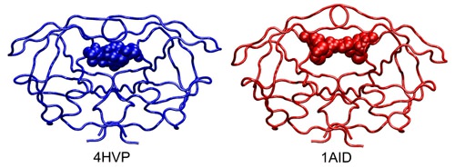
structure of the HIV-1 protease complexed with an inhibitor is shown in figure 5. The active site
structure for the bound form is significantly different from the structure of the unbound
conformation. In the bound state the flaps adopt a closed conformation acting as clamps on the
bound inhibitors or substrates, whereas in the unbound conformation the flaps are more open.
Molecular dynamics simulations can be run to sample the flexibility of the flaps and produce an
input data set of HIV-1 conformations to which PCA can be applied. A backbone-only
representation of HIV-1 has 594 atoms, which amounts to 1,782 degrees of freedom for each
conformation.
Figure 73.
Alternative conformations for HIV-1 protease. Tube representation of HIV-1 protease (PDB codes 4HVP and 1AID) bound to
different inhibitors represented by spheres. The plasticity of the binding site of the protein allows the protease to change its shape in order to accommodate ligands with widely different shapes and volumes.
Applying the PCA procedure as outlined before to a set of HIV-1 samples from simulation
produces 1,782-dimensional principal components. Since the physical interpretation of the PCs is
quite intuitive in this case, the PC coordinates can be split in groups of 3 to obtain the (x,y,z)
components for each of the 594 atoms. These components are 3-dimensional vectors that point in
the direction each atom would follow along the first PC. In figure 6 a), the per-atom components
of the first PC have been superimposed in purple.
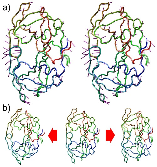
Figure 74.
First mode of motion for the HIV-1 protease. a) The purple arrows are a convenient representation of the first PC grouped every 3
coordinates -(x,y,z) for each atom- to indicate the linear path each atom would follow. Note that the "flaps" have the most important motion component, which is consistent with the simulation data. b) A reference structure (middle) can be interpolated along the first PC in a negative direction (left) or a positive one (right). Using only one degree of freedom, the flap motion can be approximated quite accurately.
Figure 6 b) shows the effect of interpolating HIV-1 conformations along the first PC, or first mode
of motion. Starting from an aligned conformation from the original data set, multiples of the first
PC can be added to produce interpolated conformations. Note that the first mode of motion
corresponds mostly to the "opening" and "closing" of the flaps, as can be inferred from the relative
magnitued of the first PC components in the flap region. Thus, interpolating in the direction of the
first PC produces an approximation of this motion, but using only one degree of freedom. This
way, the complex dynamics of the system and the 1,782 apparent degrees of freedom have been
approximated by just one, effectively reducing the dimensionality of the representation.
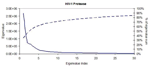
Figure 75.
The residual variance (solid line) and percentage of overall variance explained (dashed line) after each principal component.
Figure 7 (solid line) shows the residual variance left unexplained by discarding the lower-ranked
principal components. Residual variance plots always decrease, and in this case, the first PC
accounts for approximately 40% of the total variance along the motion (the dashed line shows the
percentage of total variance explained up to the given PC). Also, the first 10 PCs account for more
than 70% of the total data variance. Given the dominance of only a few degrees of freedom it is
possible to represent the flexibility of the protein in a drastically reduced search space.
Non-Linear Methods
PCA falls in the category of what is called a linear method, since mathematically, the PCs are
computed as a series of linear operations on the input coordinates. Linear methods such as PCA
work well only when the collective atom motions are small (or linear), which is hardly the case
for most interesting biological processes. Non-linear dimensionality reduction methods do exist,
but are normally much more computationally expensive and have other disadvantages as well.
However, non-linear methods are much more effective in describing complex processes using
much fewer parameters.
As a very simple and abstract example of when non-linear dimensionality reduction would be
preferred over a linear method such as PCA, consider the data set depicted in figure 8 a). The data
is apparently two-dimensional, and naively considering the data variance in this way leads to two
"important" principal components, as figure 8 b) shows. However, the data has been sampled from
a one-dimensional, but non-linear, process. Figure 8 c) shows the correct interpretation of this
data set as non-linear but one-dimensional.
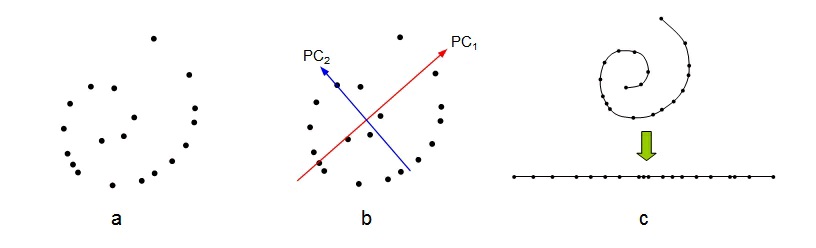
Figure 76.
Effects of dimensionality reduction on an inherently non-linear data set. a) The original data given as a two-dimensional set. b) PCA identifies two PCs as contributing significantly to explain the data variance. c) However, the inherent topology (connectivity) of the data helps identify the set as being one-dimensional, but non-linear.
Most interesting molecular processes share this characteristic of being low-dimensional but
highly non-linear in nature. For example, in the protein folding example depicted in figure 1, the
atom positions follow very complicated, curved paths to achieve the folded shape. However, the
process can still be thought of as mainly one-dimensional. Linear methods such as PCA would fail
to correctly identify collective modes of motion that do not destroy the protein when followed,
much like in the simple example of figure 8.
Several non-linear dimensionality reduction techniques exist, that can be classified as either
parametric or non-parametric.
Parametric methods need to be given a model to try to fit the data, in the form of a
mathematical function called a kernel. Kernel PCA is a variant of PCA that projects the points onto a mathematical hypersurface provided as input together with the points. When using
parametric methods, the data is forced to lie on the supplied surface, so in general this family
of methods do not work well with molecular motion data, for which the non-linearity is
unknown.
Non-parametric methods use the data itself in an attempt to infer the non-linearity from it,
much like deducing the inherent connectivity in figure 8 c). The most popular methods are
Isometric Feature Mapping (Isomap) from Tenenbaum et al. [link] and Locally Linear Embedding (LLE) from Roweis et al. [link].
The Isomap algorithm is more intuitive and numerically stable than LLE and will be discussed
next.
Isometric Feature Mapping (Isomap)
Isomap was introduced by Tenenbaum et al. [link] in 2000. It is based on an improvement over a

previous technique known as MultiDimensional Scaling (MDS). Isomap aims at capturing the
non-linearity of a data set from the set itself, by computing relationships between neighboring
points. Both MDS and the non-linear improvement will be presented first, and then the Isomap
algorithm will be detailed.
MDS. Multidimensional Scaling (see Cox et al. [link]) is a technique that produces a low-dimenisional representation for an input set of n points, where the dimensions are ordered by
variance, so it is similar to PCA in this respect. However, MDS does not require coordinates as
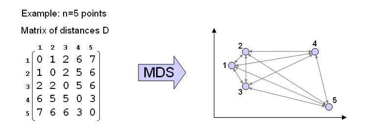
input, but rather, distances between points. More precisely, MDS requires as input a data set of
points, and a distance measure d(i,j) between any pair of points xi and xj. MDS works best when
the distance measure is a metric. MDS starts by computing all possible pairwise distances between the input points, and placing them in a matrix D so that D ij=d(i,j). The goal of MDS is to
produce, for every point, a set of n Euclidean coordinates such that the Euclidean distance between
all pairs match as close as possible the original pairwise distances D ij, as depicted in figure 9.
Figure 77.
MDS at work. A matrix of interpoint distances D is used to compute a set of Euclidean coordinates for each of the input points.
If the distance measure between points has the metric properties as explained above, then n
Euclidean coordinates can always be found for a set of n points, such that the Euclidean distance
between them matches the original distances. In order to obtain these Euclidean coordinates, such
coordinates are assumed to have a mean of zero, i.e., they are centered. In this way, the matrix of
pairwise distances D can be converted into a matrix of dot products by squaring the distances and
performing a "double centering" on them to produce the matrix B of pairwise dot products:
Let's assume that n Euclidean coordinates exist for each data point and that such coordinates can


be placed in a matrix X. Then, multiplying X by its transpose should equal the matrix B of dot
products computed before. Finally, in order to retrieve the coordinates in the unknown matrix X,
we can perform an SVD of B which can be expressed as:
Where the left and right singular vectors coincide because B is a symmetric matrix. The diagonal
matrix of eigenvalues can be split into two identical matrices, each having the square root of the
eigenvalues, and by doing this a solution for X can be found:
Since X has been computed through an SVD, the coordinates are ordered by data variance like in
PCA, so the first component of X is the most important, and so on. Keeping this in mind, the
dimensionality reduction can be performed by ignoring the higher dimensions in X and only
keeping the first few, like in PCA.
Geodesic distances. The notion of "geodesic" distance was originally defined as the length of a
geodesic path, where the geodesic path between two points on the surface of the Earth is
considered the "shortest path" since one is constrained to travel on the Earth's surface. The
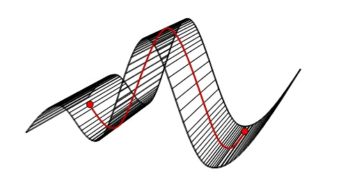
concept of geodesic distance can be generalized to any mathematical surface, and defined as "the
length of the shortest path between two points that lie on a surface, when the path is constrained to
lie on the surface." Figure 10 shows a schematic of this generalized concept of geodesic path and
distance.
Figure 78.
Geodesic distance. The geodesic distance between the two red points is the length of the geodesic path, which is the shortest path between the points, that lies on the surface.
The Isomap algorithm. The Isomap method augments classical MDS with the notion of geodesic
distance, in order to capture the non-linearity of a data set. To achieve its goal, Isomap uses MDS
to compute few Euclidean coordinates that best preserve pairwise geodesic distances, rather than
direct distances. Since the coordinates computed by MDS are Euclidean, these can be plotted on a
Cartesian set of axes. The effect of Isomap is similar to "unrolling" the non-linear surface into a
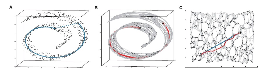
natural parameterization, as depicted in figure 11. Isomap approximates the geodesic distances
from the data itself, by first building a neighborhood graph for the data. A neighborhood graph
consists of the original set of points, together with a connection between "neighboring" points
(neighboring points are defined as the closest points to a given point, as determined by the
distance measure used) as shown in figure 11-b. After the neighborhood graph has been built, it
can be used to approximate the geodesic distance between all pairs of points as the shortest path
distance along the graph (red path in figure 11-b). Naturally, the sampling of the data set has to be
enough to capture the inherent topology of the non-linear space for this approximation to work.
MDS then takes these geodesic distances and produces the Euclidean coordinates for the set.
Figure 11-c shows two Euclidean coordinates for each point in the example.
Figure 79.
Isomap at work on the "swiss roll" data set. a) The input data is given as three-dimensional, but is really two-dimensional in nature. b) Each point in the data set is connected to its neighbors to form a neighborhood graph, overlaid in light grey. Geodesic distances are approximated by computing shortest paths along the neighborhood graph (red). c) MDS applied to the geodesic distances has the effect of "unrolling" the swiss roll into its natural, two-dimensional parameterization. The neighborhood graph has been overlaid for comparison. Now, the Euclidean distances (in blue) approximate the original geodesic distances (in red).
The Isomap method can be put in algorithmic form in the following way:
The Isomap algorithm
1. Build the neighborhood graph. Take all input points and connect each point to the closest
ones according to the distance measure used. Different criteria can be used to select the closest
neighbors, such as the k closest or all points within some threshold distance.
2. Compute all pairwise geodesic distances. These are computed as the shortest paths on the
neighborhood graph. Efficient algorithms for computing all-pairs-shortest-paths exist, such as
Dijkstra's algorithm. All geodesic distances can be put in a matrix D.
3. Perform MDS on geodesic distances. Take the matrix D and apply MDS to it. That is, apply
the double-centering formula explained above to produce B, and compute the low-dimensional
coordinates by computing B's eigenvectors and eigenvalues.
The Isomap algorithm captures the non-linearity of the data set automatically, from the data itself.
It returns a low-dimensional projection for each point; these projections can be used to understand
the underlying data distribution better. However, Isomap does not return "modes of motion" like
PCA does, along which other points can be interpolated. Also, Isomap is much more expensive
than PCA, since building a neighborhood graph and computing all-pairs-shortest-paths can have
quadratic complexity on the number of input points. Plus, ther is the hidden cost of the distance
measure itself, which can also be quite expensive. Regardless of its computational cost, Isomap
has proven extremely useful in describing non-linear processes with few parameters. In particular,
the work in Das et al. [link] applied Isomap successfully to the study of a protein folding reaction.
In order to apply Isomap to a set of molecular conformations (gathered, for example, through
molecular dynamics simulations) all that is needed is a distance measure between two
conformations. The most popular distance measure for conformations is lRMSD, discussed in the
module Molecular Distance Measures. There is no need to pre-align all the conformations in this case, since the lRMSD distance already includes pairwise alignment. Thus, the Isomap algorithm
as described above can be directly applied to molecular conformations. Choosing an appropriate
value for a neighborhood parameter (such as k) may require a bit of experience, though, and it
may depend on the amount and variability of the data. It should be noted that now, the shape of the
low-dimensional surface where we hypothesize the points lie is unknown to us. In the swiss roll
example above, it was obvious that the data was sampled from a two-dimensional surface. For
molecular data, however, we do not know, a priori, what the surface looks like. But we know that
the process should be low-dimensional and highly non-linear in nature. Of course, the distance
measure used as an underlying operation has an impact on the final coordinates as well. The
validation of the Isomap method using the lRMSD distance on protein folding data was done in
Das et al. [link], where a statistical analysis method was used to prove its usefulness.
Figure 12 shows the results of applying Isomap to the same molecular trajectory used for the CV-
N example in the PCA section. CV-N is a protein that is known to have an "intermediate" state in
the folding mechanism, and it is also known to fold through a very ordered process following a
well-defined "folding route".
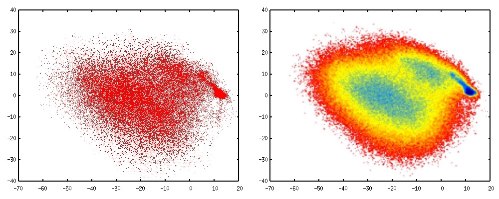
Figure 80.
The first two Isomap coordinates for the CV-N protein folding trajectory. Left: the projection of each simulated point onto the first two low-dimensional coordinates. Right: A free-energy (probability) surface computed using the Isomap coordinates.
The free-energy plot in figure 12 (right) clearly shows the superior quality of the Isomap
coordinates when compared with PCA. Isomap clearly identifies the CV-N intermediate (seen as a
free-energy minimum in blue) in between the unfolded and folded states. Also, the highest
probability route connecting the intermediate to the folded state is clearly seen in this rendering.
The PCA coordinates did not identify an itermediate or a folding route, since the PCA coordinates
are simply a linear projection of the original coordinates. Isomap, on the contrary, finds the
underlying connectivity of the data and always returns coordinates that clearly show the
progression of the reaction along its different stages.
The Isomap procedure can be applied to different molecular models. As another, smaller example,
consider the Alanine Dipeptide molecule shown in figure 13 (left). This is an all-atom molecule
that has been studied thoroughly and is known to have two predominant shapes: an "extended"
shape (also called C5 and a variant called PII) and a "helical" shape (also called alpha, with three
variants: right-handed, P-like, and left-handed). The application of the Isomap algorithm to this
molecule, without any bias by a priori known information, yields the low-dimensional coordinates
on the left of figure 13 (shown again as a free-energy plot). The first two coordinates (top right)
are already enough to identify all five major states of the peptide, and the possible transitions
between them. Applying PCA to such a simple molecule yields comparable results (not shown),
but PCA cannot differentiate the left-handed helix shape from the right-handed one. Only the
geodesic formulat