solvent molecules, however, is a computational cost that most methods try to avoid. Usually the
solvent model is separate from the energy function. There are several different ways of
approximating solvent interactions including the Generalized Born Model and the Poisson-
Boltzmann method. Most force fields do not have an explicit solvent term.
Other terms that describe the interaction between bonds and angles, angles and torsions and so on
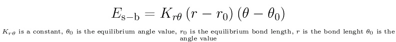
are included in some force fields. For example to model the interaction between bonds and angles:
Figure 98.
A potential energy term depending on both bond lengths and angles.
Parameters
All of the terms presented above include one or more atom-type-dependent constants, or
parameters. Determining these parameters is the major problem in developing a new potential
function. These parameters are typically found by fitting calculated results to experimental data.
Detailed quantum analysis of small molecules may also be used to set some constants. Regardless
of how it is determined, it is important to remember that all potential fields are approximations,
and most are best suited for some types of proteins over others.
An Example: The CHARMM All-Atom Empirical Potential
CHARMM (Chemistry at HARvard Macromolecular Mechanics) refers to both a program for
macromolecule dynamics and mechanics and the energy function developed for use in that
program. CHARMM is a popular force field used mainly for the study of macromolecules. In the
most recent version, the parameters were created using experimental data and supplemented with
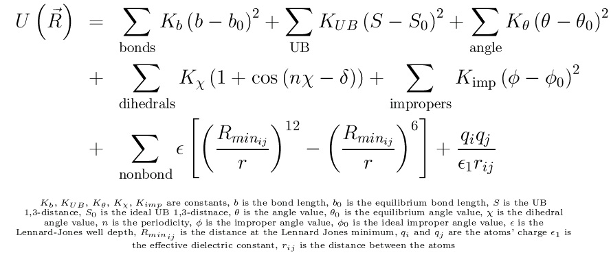
ab initio results. The CHARMM energy function has the form:
Figure 99.
The CHARMM all-atom empirical potential function
For more information on CHARMM and the CHARMM force field, please see The CHARMM
Applications of Roadmap Methods
Kinetics of Protein Folding
The two standard methods of simulating protein motion are molecular dynamics simulation (MD)
and Monte Carlo simulation (MC). In MD, a molecule or system of molecules is given an initial
set of atomic momenta, placed in a potential field, and allowed to evolve over time following
Newton's equations of motion and the forces exerted on it by the field. In MC, a series of
perturbations is applied to a single molecule. After each perturbation, if the estimated energy of
the molecule has decreased, the perturbed conformation is used for the next step of the simulation.
If the energy has increased, the perturbed conformation might be accepted, with a probability that
drops off sharply as the energy change increases. Otherwise, the perturbed conformation is
rejected and the previous conformation is perturbed again. Properly implemented MC or MD
simulations, run for long enough, should generate a series of conformations with a Boltzmann-like
distribution of structures (see the first section of this module for a reminder of what the
Boltzmann distribution looks like).
The problem with these methods is that they are very slow. A single MD simulation of a few
nanoseconds of motion for an average-size protein, performed on a cluster of processors, can take
days, and such simulations are of limited reliability due to approximations of energy and to the
extremely short time periods that can be simulated in a reasonable amount of CPU time.
Simulations must be repeated to determine what a reasonable, average behavior might look like.
Some protein rearrangement events take place on a scale of microseconds, milliseconds, or even
seconds, so a trajectory of a few nanoseconds cannot hope to capture these low-frequency events.
The field of chemical kinetics is concerned with the rate at which chemical processes take place,
and therefore, the pathways and mechanisms by which they occur. In protein biochemistry, one of
the major open questions is the protein folding problem: Given a protein, and its folded (native)
and unfolded (denatured) structures, what is the mechanism by which the protein folds into its
native state? Currently (2006), it is possible to determine in the laboratory the rate at which a
protein folds and sometimes the form of its transition state, the highest energy conformation(s) it
assumes in the process of folding. These laboratory measurements can be compared to those
inferred from simulation, and the quality of the simulation can thereby be indirectly estimated.
Roadmap-based algorithms to study this problem began with work by Latombe, Singh, and
Brutlag in 1999 [link], in which they attempted to use a PRM to find and study protein binding pockets. This work led directly to that of Song and Amato, Apaydin and Latombe, and Singal and
Pande, all presented below. Existing methods as of early 2006 are presented.
A PRM-Based Approach
The research group of Nancy Amato has been working on roadmap-based methods to study the
process of protein folding [link] [link] [link] [link]. They start with the known native structure of a protein, and incrementally find conformations more and more different from the native state,
and build a roadmap using these conformations. The goal is to find a large ensemble of pathways
between the native structure and unfolded structures, and to study these pathways and their
properties. In their work, the degrees of freedom of the protein are assumed to be the φ and ψ
backbone dihedral angles of each amino acid residue. The side chains are assumed to be rigidly
attached to the backbone. In their initial work, they generated new conformations for their
roadmaps by adjusting the backbone dihedral angles in the folded conformation randomly with
various standard deviations. This approach worked well for very small proteins, but did not scale
well.
A later sampling approach was based on counting native contacts. For the purposes of their
method, a native contact was defined as any two alpha-carbons within 7 Å of each other in the
folded state of the protein. A new conformation is generated at each step of the sampling phase of
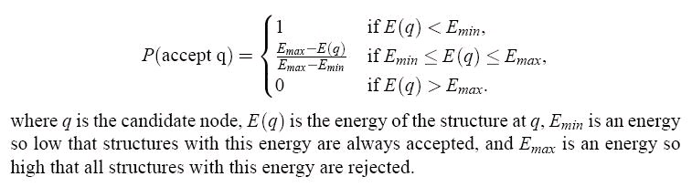
the roadmap construction by randomly perturbing some existing sample. The resulting structure
was accepted with a probability as follows:
Figure 100.
The acceptance criterion for newly sampled conformations.
The energy, E, used in this research includes a term favoring known secondary structure contacts,
and a Lennard-Jones 12-6 term as presented in the previous section. The parameters of the
Lennard-Jones term are selected to favor interactions between H and O atoms, and thus hydrogen
bonds. The energy thresholds for acceptance are decided by experiment. If accepted, a structure is
placed in a bin corresponding to the number of native contacts present, with one bin for each
possible number of native contacts from 1 to n. The procedure begins by sampling around
structures in the 100% native contacts bin (initially, just the native structure). Once the next bin,
with one fewer contacts, is full, samples are made by perturbing structures in that bin. Thus, the
sampling generally proceeds from structures with all native contacts to structures with very few
native contacts.
Once the samples are generated, an attempt is made to connect the k nearest neighbors of each
node to the node itself. A series of conformations on the line connecting the two nodes are tested,
and if their energy is below a threshold, the edge is included in the roadmap. The weight of the
edge depends on the sequence of energies of the conformations computed along the connecting
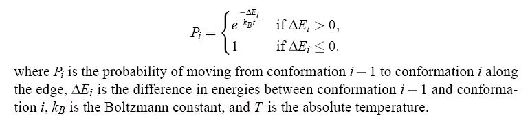
line. The probability of moving from the (i-1)th structure to the ith along the line is given by:
Figure 101.
The weight of an edge is the sum of the logarithms of the probabilities, and is intended to
represent the energetic feasibility of making the transition from the conformation represented by
one node to the next. This assumes that moving from one node in the roadmap to an adjacent one
consists of a series of move along the edge, each associated with a probability. Note that in reality,
the path taken by a protein transitioning between two structures need not be a straight line in
conformation space.
Once the roadmap is computed, the shortest paths between structures can be found using Djikstra's
algorithm, and the folding paths can be extracted and studied. In particular, the order of secondary
structure formation can be predicted by a consensus method. The order of secondary structure
formation is determined for all paths in the roadmap from unfolded to folded structures, and the
most common order is predicted as the true order of formation, which is a coarse, high-level
expression of the folding mechanism. On a set of proteins used to test their method, the predicted
formation order matched laboratory-determined formation order in all cases where it was
available. Because of the coarseness of this notion of the folding mechanism, a statistical analysis
of all pathways makes sense.
In their most recent work [link], these researchers have refined the method by which new structures are generated in the sampling phase of roadmap construction. This method is based on
rigidity analysis. For each structure, each degree of freedom is determined to be independently
flexible, dependently flexible, or rigid, using an algorithm called the Pebble Game [link].
Independently flexible degrees of freedom rotate with no deterministic effect on others.
Dependently flexible degrees of freedom force other degrees of freedom to change in a set way.
Rigid degrees of freedom are essentially locked in place unless the constraints change. In
perturbing an existing structure to generate a new sample, degrees of freedom are perturbed with a
strong bias towards perturbing independently flexible degrees of freedom and against perturbing
rigid degrees of freedom. Because the new structures are generated by physically realistic
motions, it is expected that they will generally be lower energy and more representative of real
structures than if they were generated by completely random perturbation of the degrees of
freedom.
In practice, rigidity sampling appears to allow construction of high-quality roadmaps with many
fewer samples than were necessary without it. It thus improves the overall efficiency of
calculating protein behavior using this roadmap method.
Stochastic Roadmap Simulations
Numerous variants of MD and MC have been developed in an effort to speed up the process or
focus the simulations on particular motions of interest. One method, called the Stochastic
Roadmap Simulation (SRS) [link] [link] [link] [link] uses a PRM-like structure to approximate a large number of simultaneous MC simulations very rapidly, allowing the analysis of an
ensemble of trajectories. This method followed very directly from the first roadmap studies of
molecular properties by Singh and Latombe.
The SRS method proceeds as follows:
N samples are made uniformly at random by selection of a random value for each dihedral
angle.
The k nearest neighbors for each sample are found.
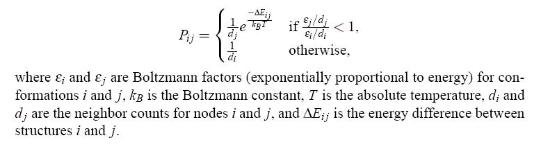
For each sample, a transition probability is calculated to each of its nearest neighbors,
depending on their energy difference as follows:
Figure 102.
Transition probabilities for SRS.
The energy, E, in this method is based on the hydrophobic-polar (H-P) energy model, and
includes two terms, one favoring hydrophobic interactions, and the other depending on the
solvent-excluded volume. Note the difference between the transition probabilities calculated by
this method and those calculated by the method presented in the previous section. These
probabilities depend only on the energies of the endpoints of an edge, whereas those of the
other method depend on the energy along the path between the endpoints. The probabilities of
the SRS method are faster to calculate, and, assuming that the system is at equilibrium, more
likely to be consistent with the actual distribution of conformations.
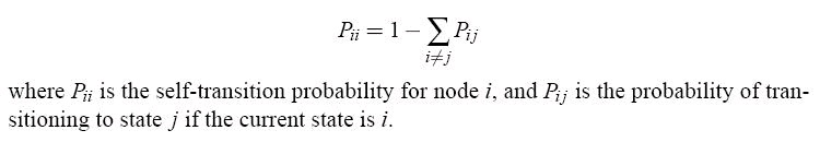
Each sample is given a self-transition probability as follows, so that the sum of outgoing edge
probabilities for each node is 1:
Figure 103.
Self-transition probabilities ensure that the total transition probability is 1.
The transition probabilities are defined as they are to be consistent with a Boltzmann-like
distribution of energies, and therefore with standard Monte Carlo simulation probabilities. The
authors demonstrated that each continuous path in the roadmap may be interpreted as a Monte
Carlo simulation, and that, if a very large number of samples and edges are made, the aggregate
behavior of these Monte Carlo simulations can be analyzed to estimate properties of the protein
such as folding rates and transition states. Essentially, SRS is a way to generate large amounts
of Monte Carlo simulation data in a short time. The developers or this method have provided a
proof that, for a sufficiently large SRS and a sufficiently long Monte Carlo simulation, the
distribution of conformations is expected to be equal.
To study protein folding using SRS, we observe that some set of nodes in the roadmap represent
conformations in or very close to the folded state (native structure). We will refer to this set of
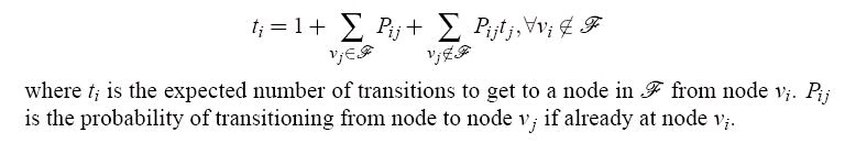
nodes as F. For every node in the roadmap, we can compute an expected number of state
transitions (or Monte Carlo steps) to go from that state to a node in F, with the base case that any
node in F is defined to be at distance 0 from F. Given a precomputed SRS, we can compute this
statistic for each node as follows:
Figure 104.
The expected number of transitions to reach a node in the folded state starting from node i.
This implies a system of linear equations on the variables ti. This system can be solved by an
iterative numerical method such as Jacobi iteration. The solution is an estimate for each node of
the average number of Monte Carlo steps necessary to achieve a folded conformation.
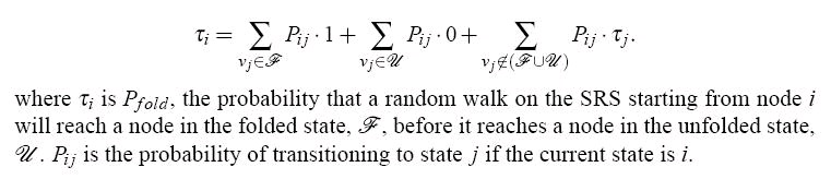
We can also define a set of nodes representing conformations close to the stable denatured state of
the protein as the unfolded state, U. Given both of the sets U and F, we can define a quantity called
the transmission coefficient, τ, for each node. The transmission coefficient expresses the
probability that a structure at a particular node will proceed to a state in F before it reaches a state
in U--in other words, it is the probability that a given structure will fold before it unfolds. This is
often called the folding probability, or Pfold, in more recent research. The quantity, τ, is
calculated for each node using the following relation:
Figure 105.
The folding probability for a node i. This is the probability than a simulation starting at node i reaches a folded state before reaching an unfolded state.
As before, this relation implies a system of linear equations, this time on τi, the τ-value of each
node. Again, it can be solved iteratively, and the result is a Pfold (τ) value for each node. Pfold is
an interesting statistic in studying the mechanism of protein folding because structures with a true
(as opposed to simulation-derived) Pfold of 0.5 have equal probability of going to the folded or
unfolded states, and therefore each one is the highest energy structure on some folding pathway.
These are the structures that constitute the transition state ensemble (TSE) of the protein, and
study of these structures may provide insight into the mechanism by which the protein folds.
Markovian State Models
Markovian State Models (MSM) [link] [link] are roadmaps constructed by running many molecular simulations (Monte Carlo and molecular dynamics) and merging the trajectories. The
method starts with a simulation that runs from the folded to unfolded state. It then picks a
structure at random (call it c) from this trajectory and run a new simulation. If this new simulation
reaches the unfolded state, then the next trajectory from which we will pick a structure will
consist of the old trajectory from the folded state to c, and the new trajectory from c to the
unfolded state. If the new trajectory reaches the folded state, we do the opposite. If neither
happens in a reasonable time, we reject the new trajectory and start over. This is repeated a set
number of times, and each time a trajectory is accepted, all states from the new part of the
trajectory are added to the growing roadmap as nodes, and each transition from the trajectory is
added as an edge. When it is added, each edge is labeled with a transition probability of 1 and a
transition time equal to the timestep of the simulation.
The goal of this method is to move roadmap methods closer to MD and MC simulations, and in
particular to incorporate a notion of time, which follows from the use of simulation techniques in
the sampling of new conformations.
Once all of the simulations have been run, nodes that are within some cutoff distance of each other
by some similarity metric must be merged. To merge two nodes, one node is removed, and its
edges are transferred to the other node. If this results in two edges between the same pair of nodes,
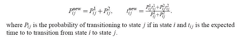
the transition probabilities and times are defined as follows:
Figure 106.
Expressions for new transition probabilities and transition times when merging nodes in constructing a MSM.
Once all merges are complete, the transition probabilities for each edge are normalized to the
range [0,1] such that the sum of all outgoing edge probabilities from a node is 1. Given the
roadmap, Pfold values and folding times can be calculated using the edge probabilities and step
times. The approach is the same as with SRS: A system of equations is set up, but instead of Pfold,
the value of interest is the expected time for a simulation starting at node i to reach a folded state,
called the mean first passage time (MFPT). The system of equations is solved using standard
numerical methods, as with SRS. On tests of a small protein, called tryptophan zipper beta
hairpin, or TZ2, the predicted folding rates agreed well with experiment.
An important fact of all roadmap methods that attempt to extrapolate properties of the entire
protein folding landscape is that there is inherent sampling error. The energy landscape of a
protein is a continuous function, which roadmap methods attempt to approximate through discrete
sampling. The researchers who developed the MSM method also developed a method to estimate
the error of the folding rates estimated based on MSMs [link]. While a complete description is beyond the scope of this module, the details are available in the 2005 paper by Singhal and Pande
linked in the Recommended Reading section below. The error analysis allows them to generate a
probability distribution for the folding times for each node in the MSM. Useful in its own right
because it gives us an idea of how confident we can be in folding times generated by a given
MSM, this analysis is especially useful for focusing sampling during the generation of an MSM.
The variance of the distribution of the folding time for each node provides an estimate of the
error. If at each stage of simulation instead of choosing a node at random to start the next
simulation, we select the node with the greatest contribution to our estimate of the error in folding
time, we effectively focus our efforts where they will decrease the error most. In this way, MSMs
with less overall error may be generated with using simulations.
Protein-Ligand Docking Pathways and Kinetics
So far, we have looked at applications of roadmap methods that deal with the single-body problem
of protein folding. The first use of roadmaps in molecular modeling, however, was to study the
two-body system of protein-ligand docking. The docking problem itself is, given a small molecule
and a protein, to predict whether they will bind to form a complex, and if so, what will be the
geometry and stability (binding affinity) of this complex. This problem is path-independent, and
so does not lend itself to motion planning approaches. Roadmaps can be used, however, to study
the question of how a ligand reaches or exits the binding pocket of a protein, what the energy
profile of this process looks like, and the rate at which the ligand binds and dissociates.
Typically, in modeling protein-ligand docking with a roadmap, the protein is held rigid and
induces a force field in which the ligand is free to rotate, translate, and change conformation. The
first work in this area, by Latombe, Singh, and Brutlag [link], led a few years later to the SRS
framework. An SRS for ligand docking pathways can be constructed be starting with the ligand in
the bound state, and generating samples for its conformation, location, and orientation in, around,
and outside the binding pocket of the protein. These paths can then be studied individually to
examine features of the binding process, or as an aggregate to get properties such as binding
affinity or escape time, which is represented in an SRS by the weight of paths away from the
bound state.
To validate their method for studying docking, the developers of SRS showed [link] that the escape times (in Monte Carlo steps) calculated for ligands leaving proteins with particular
mutations in their binding sites were consistent with the expected effect of the mutations:
Mutations expected to increase the binding affinity led to longer escape times, and mutations
expected to decrease the binding affinity led to shorter escape times. They also showed that SRS
could be used to distinguish between the binding site of the protein and other pockets on its
surface. Ligands had significantly greater estimated escape times from the true binding site than
from spurious ones.
Cortes et al. [link] developed a tree-based sampling method for studying protein-ligand docking
pathways. The algorithm is based on the dynamic-domain RRT planner (see Robotic Path
Planning and Protein Modeling for an introduction to RRTs and other tree-based motion
planners), in which, when sampling a random point toward which to expand, the location of that
point is restricted to be within some distance of the existing tree, rather than anywhere in the
whole space. The sampling method is based on the geometry of the system being studied: The
major factors contributing to the energy of a conformation are reduced to geometric criteria.
Hydrogen bonds and hydrophobic interactions are modeled by distance constraints. Steric clash is
handled by treating atoms as hard spheres and performing collision checks using a fast collision
checker called BioCD, developed by the same research group. Only structures satisfying all
geometric constraints are subjected to an energy minimization procedure. The geometric
constraints help ensure that structures to be added to the tree are already fairly low-energy,
ensuring that the minimization can be done quickly, and that time is not wasted minimizing
unrealistic structures.
This work was applied to studying the enantioselectivity of various proteins. Enantiomers are
molecules that are non-superimposable mirror images of each other. Although they contain the
same atom types and connectivity, enantiomers of a given chemical cannot be interconverted
without breaking and reforming bonds. Molecules may contain multiple sites where this kind of
asymmetry exists, in which case the molecule may exist as a whole family of diasteroemers.
Most biological molecules have at least one asymmetric c