Solution : We can proceed to find the magnitude of total acceleration by first finding the
expression of velocity. Here, velocity is given as :
Since acceleration is higher order attribute, we obtain its expression by differentiating the
expression of velocity with respect to time :
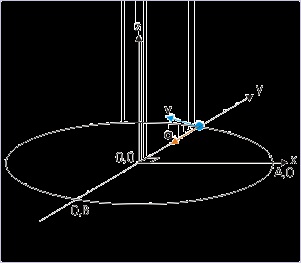
It is obvious that acceleration is one dimensional. It is evident from the data given also. The
balloon moving with constant vertical velocity has no acceleration in y-direction. The speed of
the balloon in x-direction, however, keeps changing with height (time) and as such total
acceleration of the balloon is in x-direction. The magnitude of total acceleration is :
Figure 4.112. Motion of a balloon
The acceleration of the balloon has two components in mutually perpendicular directions.
Thus, we see that total acceleration is not only one dimensional, but constant as well.
However, this does not mean that component accelerations viz tangential and normal


accelerations are also constant. We need to investigate their expressions. We can obtain
tangential acceleration as time rate of change of the magnitude of velocity i.e. the time rate of
change of speed. We, therefore, need to first know an expression of the speed. Now, speed is :
Differentiating with respect to time, we have :
In order to find the normal acceleration, we use the fact that total acceleration is vector sum of
two mutually perpendicular tangential and normal accelerations.
a 2 = a 2 T + a 2 N
Nature of motion
Example 4.63.
Problem : The coordinates of a particle moving in a plane are given by x = A cos(ωt) and y =
B sin (ωt) where A, B (< A) and “ω” are positive constants of appropriate dimensions. Prove
that the velocity and acceleration of the particle are normal to each other at t = π/2ω.
Solution : By differentiation, the components of velocity and acceleration are as given under :
The components of velocity in “x” and “y” directions are :
The components of acceleration in “x” and “y” directions are :


At time,
and
. Putting this value in the component expressions, we have :
Figure 4.113. Motion along elliptical path
Velocity and acceleration are perpendicular at the given instant.
⇒ vx = – A ω sin ω t = – A ω sin π / 2 = – A ω
⇒ vy = B ω cos ω t = B ω cos π / 2 = 0
⇒ ax = – A ω 2 cos ω t = – A ω 2 cos π / 2 = 0
⇒ a y = – B ω 2 sin ω t = – b ω 2 sin π / 2 = – B ω 2
The net velocity is in negative x-direction, whereas net acceleration is in negative y-direction.
Hence at
, velocity and acceleration of the particle are normal to each other.
Example 4.64.
Problem : Position vector of a particle is :
Show that velocity vector is perpendicular to position vector.
Solution : We shall use a different technique to prove as required. We shall use the fact that
scalar (dot) product of two perpendicular vectors is zero. We, therefore, need to find the
expression of velocity. We can obtain the same by differentiating the expression of position
vector with respect to time as :


To check whether velocity is perpendicular to the position vector, we take the scalar product
of r and v as :
This means that the angle between position vector and velocity are at right angle to each other.
Hence, velocity is perpendicular to position vector.
Displacement in two dimensions
Example 4.65.
Problem : The coordinates of a particle moving in a plane are given by x = A cos(ω t) and y =
B sin (ω t) where A, B (<A) and ω are positive constants of appropriate dimensions. Find the
displacement of the particle in time interval t = 0 to t = π/2 ω.
Solution : In order to find the displacement, we shall first know the positions of the particle at
the start of motion and at the given time. Now, the position of the particle is given by
coordinates :
x = A cos ω t
and
y = B sin ω t
At t = 0, the position of the particle is given by :
⇒ x = A cos ( ω x 0 ) = A cos 0 = A
⇒ y = B sin ( ω x 0 ) = B sin 0 = 0
At
, the position of the particle is given by :
⇒ x = A cos ( ω x π / 2 ω ) = A cos π / 2 = 0
⇒ y = B sin ( ω x π / 2 ω ) = a sin π / 2 = B
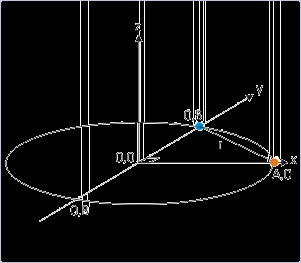

Figure 4.114. Motion along an elliptical path
The linear distance equals displacement.
Therefore , the displacement in the given time interval is :
Transformation of graphs*
Transformation of graphs means changing graphs. This generally allows us to draw graphs of
more complicated functions from graphs of basic or simpler functions by applying different
transformation techniques. It is important to emphasize here that plotting a graph is an extremely
powerful technique and method to know properties of a function such as domain, range,
periodicity, polarity and other features which involve differentiability of a function. Subsequently,
we shall see that plotting enables us to know these properties more elegantly and easily as
compared to other analytical methods.
Graphing of a given function involves modifying graph of a core function. We modify core
function and its graph, applying various mathematical operations on the core function. There are
two fundamental ways in which we operate on core function and hence its graph. We can either
modify input to the function or modify output of function.
Broad categories of transformation
Transformation applied by modification to input
Transformation applied by modification to output
Transformation applied by modulus function
Transformation applied by greatest integer function


Transformation applied by fraction part function
Transformation applied by least integer function
We shall cover first transformation in this module. Others will be taken up in other modules.
Important concepts
Graph of a function
It is a plot of values of function against independent variable x. The value of function changes in
accordance with function rule as x changes. Graph depicts these changes pictorially. In the current
context, both core function and modified function graphs are plotted against same independent
variable x.
Input to the function
What is input to the function? How do we change input to the function? Values are passed to the
function through argument of the function. The argument itself is a function in x i.e. independent
variable. The simplest form of argument is "x" like in function f(x). The modified arguments are
"2x" in function f(2x) or "2x-1" in function f(2x-1). This changes input to the function. Important
to underline is that independent variable x remains what it is, but argument of the function
changes due to mathematical operation on independent variable. Thus, we modify argument
though mathematical operation on independent variable x. Basic possibilities of modifying
argument i.e. input by using arithmetic operations on x are addition, subtraction, multiplication,
division and negation. In notation, we write modification to the input of the function as :
These changes are called internal or pre-composition modifications.
Output of the function
A modification in input to the graph is reflected in the values of the function. This is one way of
modifying output and hence corresponding graph. Yet another approach of changing output is by
applying arithmetic operations on the function itself. We shall represent such arithmetic
operations on the function as :
These changes are called external or post-composition modifications.


Arithmetic operations
Addition/subtraction operations
Addition and subtraction to independent variable x is represented as :
The notation represents addition operation when c is positive and subtraction when c is negative.
In particular, we should underline that notation “bx+c” does not represent addition to independent
variable. Rather it represents addition/ subtraction to “bx”. We shall develop proper algorithm to
handle such operations subsequently. Similarly, addition and subtraction operation on function is
represented as :
Again, “af(x) + d” is addition/ subtraction to “af(x)” not to “f(x)”.
Product/division operations
Product and division operations are defined with a positive constant for both independent variable
and function. It is because negation i.e. multiplication or division with -1 is a separate operation
from the point of graphical effect. In the case of product operation, the magnitude of constants (a
or b) is greater than 1 such that resulting value is greater than the original value.
The division operation is eqivalent to product operation when value of multiplier is less than 1. In
this case, magnitude of constants (a or b) is less than 1 such that resulting value is less than the
original value.
Negation
Negation means multiplication or division by -1.
Effect of arithmetic operations
Addition/ subtraction operation on independent variable results in shifting of core graph along x-
axis i..e horizontally. Similarly, product/division operations results in scaling (shrinking or
stretching) of core graph horizontally. The change in graphs due to negation is reflected as
mirroring (across y–axis) horizontally. Clearly, modifications resulting from modification to


input modifies core graph horizontally. Another important aspect of these modification is that
changes takes place opposite to that of operation on independent variable. For example, when “2”
is added to independent variable, then core graph shifts left which is opposite to the direction of
increasing x. A multiplication by 2 shrinks the graph horizontally by a factor 2, whereas division
by 2 stretches the graph by a factor of 2.
On the other hand, modification in the output of function is reflected in change in graphs along y-
axis i.e. vertically. Effects such as shifting, scaling (shrinking or stretching) or mirroring across x-
axis takes place in vertical direction. Also, the effect of modification in output is in the direction
of modification as against effects due to modifications to input. A multiplication of function by a
positive constant greater than 1, for example, stretches the graph in y-direction as expected. These
aspects will be clear as we study each of the modifications mentioned here.
Forms of representation
There is a bit of ambiguity about the nature of constants in symbolic representation of
transformation. Consider the representation,
In this case "a", "b", "c" and "d" can be either positive or negative depending on the particular transformation. A positive "d" means that graph is shifted up. On the other hand, we can specify
constants to be positive in the following representation :
The form of representation appears to be cumbersome, but is more explicit in its intent. It delinks
sign from the magnitude of constants. In this case, the signs preceding positive constants need to
be interpreted for the nature of transformation. For example, a negative sign before c denotes right
horizontal shift. It is, however, clear that both representations are essentially equivalent and their
use depends on personal choice or context. This difference does not matter so long we understand
the process of graphing.
Transformation of graph by input
Addition and subtraction to independent variable
In order to understand this type of transformation, we need to explore how output of the function
changes as input to the function changes. Let us consider an example of functions f(x) and f(x+1).
The integral values of inedependent variable are same as integral values on x-axis of coordinate
system. Note that independent variable is plotted along x-axis as real number line. The integral
x+1 values to the function f(x+1) - such that input values are same as that of f(x) - are shown on a
separate line just below x-axis. The corresponding values are linked with arrow signs. Input to the

function f(x+1) which is same as that of f(x) corresponds to x which is 1 unit smaller. It means
graph of f(x+1) is same as graph of f(x), which has been shifted by 1 unit towards left. Else, we
can say that the origin of plot (also x-axis) has shifted right by 1 unit.
Figure 4.115. Shifting of graph parallel to x-axis
Each element of graph is shifted left by same value.
Let us now consider an example of functions f(x) and f(x-2). Input to the function f(x-2) which is
same as that of f(x) now appears 2 unit later on x-axis. It means graph of f(x-2) is same as graph
of f(x), which has been shifted by 2 units towards right. Else, we can say that the origin of plot
(also x-axis) has shifted left by 2 units.
Figure 4.116. Shifting of graph parallel to x-axis
Each element of graph is shifted right by same value.
The addition/subtraction transformation is depicted symbolically as :
If we add a positive constant to the argument of the function, then value of y at x=x in the new
function y=f(x+|a|) is same as that of y=f(x) at x=x-|a|. For this reason, the graph of f(x+|a|) is
same as the graph of y=f(x) shifted left by unit “a” in x-direction. Similarly, the graph of f(x-|a|)
is same as the graph of y=f(x) shifted right by unit “a” in x-direction.
1 : The plot of y=f(x+|a|); is the plot of y=f(x) shifted left by unit “|a|”.
2 : The plot of y=f(x-|a|); is the plot of y=f(x) shifted right by unit “|a|”.
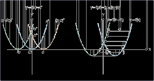
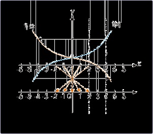
We use these facts to draw graph of transformed function f(x±a) by shifting graph of f(x) by unit
“a” in x-direction. Each point forming the plot is shifted parallel to x-axis (see quadratic graph
showm in the of figure below). The graph in the center of left figure depicts monomial function
y = x 2 with vertex at origin. It is shifted right by “a” units (a>0) and the function representing
shifted graph is y = ( x − a )2 . Note that vertex of parabola is shifted from (0,0) to (a,0). Further, the graph is shifted left by “b” units (b>0) and the function representing shifted graph is
y = ( x + b )2 . In this case, vertex of parabola is shifted from (0,0) to (-b,0).
Figure 4.117. Shifting of graph parallel to x-axis
Each element of graph is shifted by same value.
Example 4.66.
Problem : Draw graph of function 4 y = 2 x .
Solution : Given function is exponential function. On simplification, we have :
⇒ y = 2 – 2 X 2 x = 2 x – 2
Here, core graph is y = 2 x . We draw its graph first and then shift the graph right by 2 units to
get the graph of given function.
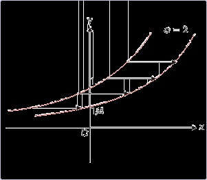

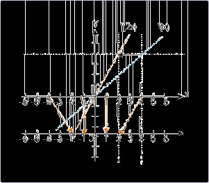
Figure 4.118. Shifting of exponential graph parallel to x-axis
Each element of graph is shifted by same value.
Note that the value of function at x=0 for core and modified functions, respectively, are :
⇒ y = 2 x = 20 = 1
Multiplication and division of independent variable
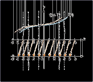
Let us consider an example of functions f(x) and f(2x). The integral values of independent
variable are same as integral values on x-axis of coordinate system. Note that independent
variable is plotted along x-axis as real number line. The integral 2x values to the function f(2x) -
such that input values are same as that of f(x) - are shown on a separate line just below x-axis. The
corresponding values are linked with arrow signs. Input to the function f(2x) which is same as that
of f(x) now appears closer to origin by a factor of 2. It means graph of f(2x) is same as graph of
f(x), which has been shrunk by a factor 2 towards origin. Else, we can say that x-axis has been
stretched by a factor 2.

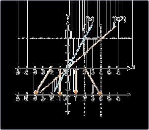

Figure 4.119. Multiplication of independent variable
The graph shrinks towards origin.
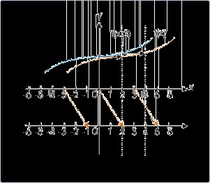
Let us consider another example of functions f(x) and f(x/2). The integral values of independent
variable are same as integral values on x-axis of coordinate system. Note that independent
variable is plotted along x-axis as real number line. The integral x/2 values to the function f(x/2) -
such that input values are same as that of f(x) - are shown on a separate line just below x-axis. The
corresponding values are linked with arrow signs. Input to the function f(x/2) which is same as
that of f(x) now appears away from origin by a factor of 2. It means graph of f(x/2) is same as
graph of f(x), which has been stretched by a factor 2 away from origin. Else, we can say that x-
axis has been shrunk by a factor 2.
Figure 4.120. Multiplication of independent variable
The graph stretches away from origin.
Important thing to note about horizontal scaling (shrinking or stretching) is that it takes place with
respect to origin of the coordinate system and along x-axis – not about any other point and not
along y-axis. What it means that behavior of graph at x=0 remains unchanged. In equivalent term,
we can say that y-intercept of graph remains same and is not affected by scaling resulting from
multiplication or division of the independent variable.
Negation of independent variable
Let us consider an example of functions f(x) and f(-x). The integral values of independent variable
are same as integral values on x-axis of coordinate system. Note that independent variable is
plotted along x-axis as real number line. The integral -x values to the function f(-x) - such that
input values are same as that of f(x) - are shown on a separate line just below x-axis. The

corresponding values are linked with arrow signs. Input to the function f(-x) which is same as that
of f(x) now appears to be flipped across y-axis. It means graph of f(-x) is same as graph of f(x),
which is mirror image in y-axis i.e. across y-axis.
Figure 4.121. Negation of independent variable
The graph flipped across y. -axis.
The form of transformation is depicted as :
A graph of a function is drawn for values of x in its domain. Depending on the nature of function,
we plot function values for both negative and positive values of x. When sign of the independent
variable is changed, the function values for negative x become the values of function for positive
x and vice-versa. It means that we need to flip the plot across y-axis. In the nutshell, the graph of
y=f(-x) can be obtained by taking mirror image of the graph of y=f(x) in y-axis.
While using this transformation, we should know about even function. For even function. f(x)=f(-
x). As such, this transformation will not have any implication for even functions as they are
already symmetric about y-axis. It means that two parts of the graph of even function across y-
a