


246
Microsensors
1μm
θ
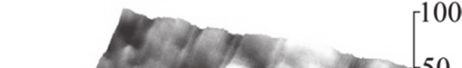
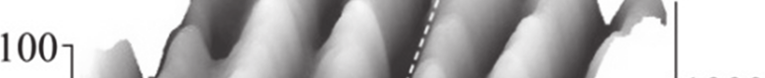
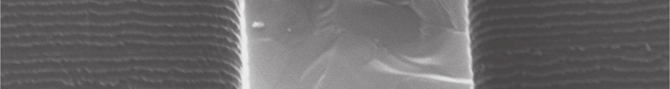
Fig. 12. Definition of fracture surface (mirror zone) angle.
] 3
sing
a mP
s ues [M
hn
IC 2
K
touge one,
tur
or z
L15R1
rac
irr 1
L15R2
d m
L15R3
ated f
L15R4
cul
ss an
L15R5
alC
h = 3.5 µm
stre 00
10
20
30
40
Angle between fracture surface and
principal stress surface [deg.]
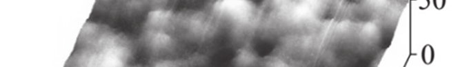
Fig. 13. Angle dependency of fracture toughness ( h = 3.5 [μm]).
5. Effective area and application to design
5.1 Effective area definition and calculation results
The stress concentration factors on the specimen surface were determined based on the
result of surface roughness measurement by AFM. As shown in Fig. 2, difference occurs in
the surface shape of the upper surface and the sidewall surface by the difference in the
manufacturing technique. Figure 14 indicates an example of the difference in surface
Strength Reliability of Micro Polycrystalline Silicon Structure
247
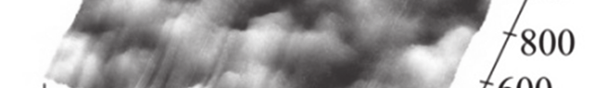
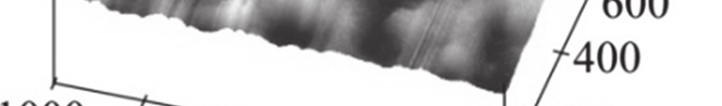
roughness of the h = 6.4 [μm] specimen obtained by AFM, and Fig. 15 indicates the example
of surface section of the scarop bottom on the sidewall surface.
Using the measurement result of the surface roughness, the stress concentration factors Kt of
the specimen were calculated. As shown in Fig. 14, the appearance present complicated
shapes, therefore FEM analysis is necessary to calculate an accurate stress concentration
factors. In this report, in order to simplify, the interference effects by the multiple notches
were ignored and the stress concentration factors Kt were determined from width ( a) and depth ( b) from the roughness measurements using the following equations supposing the
equivalent ellipse as shown in Fig. 15.
2
= 1 +
(4)
The maximum stress concentration factor Kt max which exists in a specimen based on the data
of the measured stress concentration factor is estimated using the statistics of extreme.
Figure 16 shows the extreme values probability paper. The horizontal axis is the stress
concentration factor Kt j obtained by the Eq. (4). The vertical axis is the reduced variates yj calculated by the following equation which is a formula of the statistics of extreme.
=
,
= − ln − ln
+ 1
(5)
( j = 1, 2, 3,…, n n: Number of inspections)
The approximate expression was calculated using the least square method from the
obtained distribution. The maximum stress concentration factor which substitutes the return
period T for the following equations, and Kt max exist in a specimen is estimated.
− 1
= − ln − ln
, = α
+ β
(6)
When determining the return period T, evaluation area was made equal to the effective area.
The relation between evaluation area and the return period are defined using the following
equations. ( S 0: inspection area)
+
=
,
< 10
(7)
=
,
> 10
(8)
In order to bring evaluation area close to an effective area, calculation performed repeatedly.
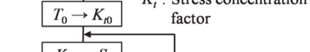
The computational procedure is as follows. Fig. 17 indicates a computational procedure outline.
1. Define T 0 by the evaluation area to the extent of the whole specimen is included enough
2. Calculate Kt i from defined T 0
3. Calculate assumed effective area Si from Eq. (1) and FEM
4. Calculate Ti, Si as evaluation area
5. Calculate Kt i+1 from Ti
6. Compare Kt i and Kt i+1. If Kt i/( Kt i+1) > 0.99, then define Si as effective area 7. If not Kt i/( Kt i+1) > 0.99, repeat the process after 3).


248
Microsensors
(a) Top surface (b) Sidewall surface
Fig. 14. Surface morphology of top and sidewall (unit: nm) ( h = 6.4 [μm]).
Fig. 15. Surface roughness example of sidewall (Fig. 14 A-B).
99.9
Top surface
%
99
ility F, ab
Sidewall
ob
surface
90
tive pr
50
ulam
10
Cu
1
0.1
1.0
1.5
2.0
2.5
Stress concentration factor K t
Fig. 16. Variation of stress concentratio
Fig. 17. Schematic diagram of deciding S
factor Kt.
from T and Kt ( h = 6.4 [μm]).


Strength Reliability of Micro Polycrystalline Silicon Structure
249
Maximum stress
Effective
Specimen
concentration factor
area
type
Kt max
S [μm2]
Top surface Sidewall surface
L15R1 1.22
1.79
4.02
L15R2 1.28
1.82
8.01
L15R3 1.34
1.84
13.7
L15R4 1.39
1.86
22.7
L15R5 1.39
1.85
22.8
L10 1.20 1.78 3.57
L15 1.21 1.78 3.47
Table 2. Result of calculations, Kt max and S ( h = 6.4 [μm]).
In this study, it calculated as initial return period value T 0 = 10000. Table 2 shows the
obtained Kt max and S.
5.2 Effective area and fracture origin
Figure 18 indicates the example in the structure of the effective area. Figure 18 shows that
the region of effective area where fracture origin may exist has extended to the specimen
sidewall. Fracture surface observation of the specimen was carried out, and the example to
which fracture origin exists in the sidewall was observed. Figure 19 shows an example. The
scattering in fracture origin is shown in Fig. 20. It turns out that fracture origin varies within
an effective area.
Fig. 18. Calculated effective area S (Specimen type: L15R5, h = 6.4 [μm]).
5.3 Application to design
Bending strength (maximum stress σmax at the time of fracture) σB and the maximum stress
concentration factor Kt max were fitted to the Eq. (1) and the effective area was determined.
Figure 21 shows the relationship between bending strength and the effective area. Average
values of the test data ( N = 8) were used for σB . The tendency bending strength becomes
small as the effective area increased can be seen.
The equation of Weibull distribution which generally took the effective volume V into
consideration same as Section 3 is shown as follows.


250
Microsensors
σ
= 1 − exp −
(9)
σ
Eq. (9) can be expressed as follows.
1
ln ln
=
ln σ − ln σ + ln
1 −
(10)
It turns out in the Eq. (10) that the effective volume V acts as a value which does not involve at the shape parameter m which shows the level of scattering. Since an effective volume did
not participate in scattering, it extrapolated to the reliability needed for a design using the
average of the shape parameter determined from the experimental result σB. In Fig. 21, an
extrapolation example in the case of F = 0.001, the relationship between σB and S are shown.
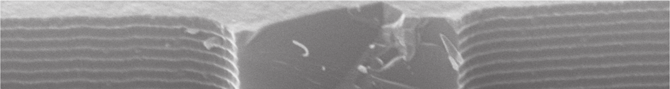
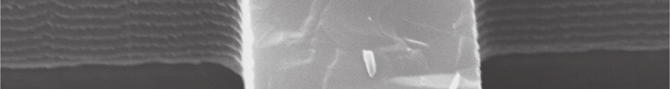
Fracture origin
2μm
0.5μm
(a) Whole fracture surface (b) Magnification of fracture origin
Fig. 19. Fracture origin on the sidewall surface ( h = 6.4 [μm]).
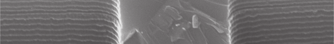
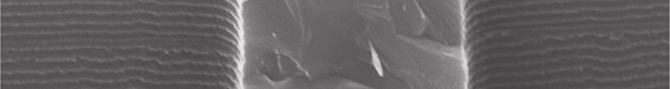
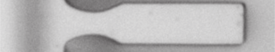
(a) Before test
(b) After test, σB = 3.15 [GPa]
5μm
(c) After test, σB = 3.41 [GPa]
(d) After test, σB = 3.67 [GPa]
Fig. 20. Variation of fracture points, Specimen type: L15R5, h = 6.4 [μm].
Strength Reliability of Micro Polycrystalline Silicon Structure
251
10
a
Experimental result, F = 0.5
, GP B 5
th
treng
Extrapolation result, F = 0.001
g sin 2
endB
11
2
5
10
20
50
100
Effective surface area S , µm2
Fig. 21. Relationship between the bending strength and effective area
6. Conclusion
In order to propose the static strength design criteria of the poly-Si structure which has a
microscopic dimension, the bending test, surface roughness measurement, FEM analysis,
the Weibull statistical analysis, statistics of extreme analysis, and fracture analysis of a
cantilever beam were conducted.
The obtained results are as follows.
1. By Weibull analysis, we found that the scatter in poly-Si bending strength made by RIE
process is smaller than that of DRIE process.
2. Poly-Si strength is scattered. It depends on surface condition, crystal or grain boundary
direction and some other.
3. The definition method of the quantitative effective area in bending cantilever beam was
shown to the poly-Si with which the surface roughness on the upper surface and the
surface of the sidewall differs.
4. Bending strength depends on the effective area definition are shown.
5. The static strength design criteria in consideration of the scattering in the strength using
two parameters, the bending strength (maximum stress at the time of fracture) and the
effective area, was proposed.
7. References
Chen, K. S.; Ayón, A. A.; Zhang X. & Spearing, S. M. (2002). Effect of Process Parameters on
the Surface Morphology and Mechanical Performance of Silicon Structures After
Deep Reactive Ion Etching (DRIE), IEEE Journal of Microelectromechanical Systems,
Vol. 11, No. 3, pp. 264-275, ISSN 1057-7157
252
Microsensors
Greek, S.; Ericson, F.; Johansson, S. & Schweitz, J.-Å. (1997). In situ tensile strength
measurement and Weibull analysis of thick film and thin film micromachined
polysilicon structures, Thin Solid Films, Vol. 292, pp. 247-254, ISSN 0040-6090
Gumbel, E. J. (1962). Statistic of Extremes, Columbia Univ. Press, New York
Hull, D. (1999). Fractography, Cambridge University Press, ISBN 0521640822, Cambridge, pp.
121-129.
Johnson, L. G. (1964). The Statistical Treatment of Fatigue Experiments, Elsevier, New York
Kahn, H.; Tayebi, N.; Ballarini, R.; Mullen R. L. & Heuer, A. H. (2000). Fracture toughness of
polysilicon MEMS devices, Sensors and Actuators A, Vol. 82, pp. 274-280, ISSN 0924-
4247
Kapels, H.; Aigner, R. & Binder, J. (2000). Fracture strength and fatigue of polysilicon
determined by a novel thermal actuator, IEEE Transactions on Electron Devices, Vol.
47, pp. 1522-1528, ISSN 0018-9383
Muhlstein, C. L.; Howe R. T. & Ritchie, R. O. (2004). Fatigue of Polycrystalline Silicon for
Microelectromechanical Systems: Crack Growth and Stability under Resonant
Loading Conditions, Mechanics of Materials, Vol. 36, pp. 13-33, ISSN 0167-6636
Murakami ,Y. Eds. (1992). Stress Intensity Factors Handbook Vol.3, Soc. Materials Sci., Japan & Pergamon Press, pp. 591-597
Najafi, K. (2000). Micromachined Micro Systems: Miniaturization Beyond Micro-electronics,
Proc. 2000 Symposium on VLSI Circuits Digest of Technical Papers, pp. 6-13
Namazu, T.; Isono Y. & Tanaka, T. (2000). Evaluation of Size Effect on Mechanical Properties
of Single Crystal Silicon by Nano-Scale Bending Test using AFM, IEEE Journal of
Microelectromechanical Systems, Vol. 9, pp. 450-459, ISSN 1057-7157
Senturia, S. D. (2000). Microsystem Design, Kluwer Academic Publishers, ISBN 0792372468,
Dordrecht
Sharpe Jr., W. N.; Jackson, K. M.; Hemker K. J. & Xie, Z. (2001). Effect of Specimen Size on
Young's Modulus and Fracture Strength of Polysilicon, IEEE Journal of
Microelectromechanical Systems, Vol. 10, pp. 317-326, ISSN 1057-7157
Son, D.; Kim, J.; Lim T. W. & Kwon, D. (2004). Evaluation of fracture properties of silicon by
combining resonance frequency and microtensile methods, Thin Solid Films, Vol.
468, pp. 167-173, ISSN 0040-6090
Tsuchiya, T.; Tabata, O.; Sakata J & Taga, Y. (1998). Specimen size effect on tensile strength
of surfacemicromachined polycrystalline silicon thin films, IEEE Journal of
Microelectromechanical Systems, Vol. 7, pp. 106-113, ISSN 1057-7157
Weibull, W. (1951). A statistical distribution function of wide applicability, Transactions
ASME Journal of Applied Mechanics, Vol. 18, pp. 293-297
12
MEMS Gyroscopes for Consumer and
Industrial Applications
Riccardo Antonello and Roberto Oboe
Dept. of Management and Engineering,
University of Padova - Vicenza branch
Italy
1. Introduction
The advent of MEMS (Micro-Electro-Mechanical-System) technology has enabled the
development of miniaturized, low-cost, low-power sensors that are currently replacing
their macroscopic scale equivalents in many traditional applications, covering industrial,
automotive, biomedical, consumer applications, etc.
Competitiveness of MEMS sensors largely resides in the miniaturization and batch fabrication
processes involved in their manufacture, which allow to cut down costs, size and power
requirements of the final device. Moreover, miniaturization opens new perspectives and
possibilities for the development of completely new class of sensors, where micro-scale
phenomena are effectively pursued to achieve results that would be unfeasible at a
macro-scale.
Several MEMS sensor typologies are either commercially available or have been presented
in technical literature since the beginning of the microsystem technology more than 30 years
ago. Pressure and acceleration sensors for the automotive industry have been among the first
MEMS devices to be produced in large scale, and they have contributed to foster the further
development of MEMS technology. Despite their maturity, these sensors are still dominating,
with their sales volume, the market of silicon-based sensors. Recently, another micro-sensor
that is becoming relevant in terms of sales volume, especially in the automotive and consumer
electronics markets, is the angular rate sensor, or gyroscope.
Alongside with accelerometers, micromachined gyroscopes can be used in several
applications that require an integrated solution for inertial sensing and motion processing
problems (Söderkvist, 1994; Yazdi et al., 1998).