Insulated areas
Either external boundaries
0
or symmetry axis
* formula extracted from [9]
Table 2. Thermo-physical parameters used in this work
In the vicinity of the surface sample, the temperature of the rarefied gas is close to the solid
one. To estimate the maximum heat loss from the surface,the gas temperature is here
voluntarily increased by 2K or 3K, depending on how far the heat source (BB) is located. For
the same reason, the screw cap temperature is also set at 2K over the solid surface one (fig.
5-b).
94
Microsensors
Owing to the plans of symmetry existing in the squared sample, the geometry of the
problem has been reduced at one eighth for the sake of finer meshing and fast computer
calculations. The whole boundaries conditions are summarized in table 2.
As shown in figure 6, the low temperature difference between the front and the back side of
the thin sample (Tsample), already obtained from 1D model is confirmed in a full 3D
modelling, whatever the thermal contact resistance value. Moreover, the temperature
difference in silicon sample is found approximately ten times higher than in copper , again
in good agreement with the 1D model..
One can also see on figure 6 the effect of Rctc on the delay to reach the steady state. As
expected, the lower is the thermal contact resistance; the faster the equilibrium regime is
reached. Note that the time expressed here could not be compared with the experiment one,
which strongly depends on the blackbody inertia. In simulations, the blackbody
temperature being immediately set at 373 K, the time evolution is only characteristic of the
thermal response of the system (cooled HFM with sample)
7,E-03
5,E-04
6,E-03
4,E-04
5,E-03
0,1
0,01
4,E-03
3,E-04
0,001
ple
ple
m
m
sa
3,E-03
sa
2,E-04
2,E-03
0,1
1,E-04
1,E-03
0,01
0,001
0,E+00
0,E+00
0
200
400
600
800
1000
0
200
400
600
800
1000
Time (s)
Time (s)
Fig. 6. Difference of front and back temperatures for Si (left) and Cu (right), at various
thermal contact resistances (in m2.K.W-1) obtained from full 3D- model
The front (TS) and the back (Tb) side temperatures of the sample presented in figure 7 are
strongly dependent on the thermal contact resistance. It is seen that the temperature of the
surface sample may be different from that of the cooling bath i.e. 278 K, even for weak thermal contact resistances.
320
315
310
310
305
305
0,1
300
) 300
0,1
(K
0,01
b
) 295
T 295
0,001
0,01
(KbT 290
0,001
290
285
285
280
280
275
275
0
200
400
600
800
1000
0
200
400
600
800
1000
Time (s)
Time (s)
Fig. 7. Simulation of the temperature time evolution at the back face of the sample for Si
(left) and Cu (right) for several thermal contact resistances, from full 3D- modelling
Simulated heat flux reaching the fluxmeter is plotted in figure 8. In the full 3D-
computations, the heat fluxes are calculated for a black body radiating at 373 K. One could


A Heat Flux Microsensor for Direct Measurements in Plasma Surface Interactions
95
easily notice that measured heat fluxes are close to the calculated ones. This result indicates
that thermal contact resistance values are in the range 10-3 to 10-1 m2.K.W-1, which is in good
agreement with values given in literature for solid-solid thermal contact resistances [6].
77
18
70
63
15
1
56
1,E-01
)
1
)
W 49
12
W
1,E-02
m
1,E-01
( 42
1,E-03
1,E-02
(m
9
flux
1,E-05
35
1,E-03
flux
eat
at
28
e
H
1,E-05
H
6
21
14
3
7
0
0
0
200
400
600
800
1000
0
200
400
600
800
1000
Time (s)
Time (s)
Fig. 8. Simulation of heat flux time evolution at the HFM surface for Si (left) and Cu (right)
samples, at various thermal contact resistances (in m2.K.W-1), from full 3D- modelling
It is interesting to compare heat fluxes deduced from experimental curves with those
calculated by 3D-simulations in similar conditions. This is summarized in table 3.
3D simulations for T
Samples T
BB = 373K
BB (°C)
Experiments
Rctc (m2.K.W-1) =
10-1 10-2 10-5
363K 12.5
mW
Copper
13 mW
17 mW
17.5 mW
393K 16
mW
363K 53
mW
Silicon
21 mW
63 mW
74 mW
393K 92
mW
Table 3. Comparisons of measured and 3D simulated heat fluxes (values given for saturation
states) for Cu and Si samples
2.3 Comparison with other heat flux probes
Since the 1960s many authors tested various techniques to measure the energy influx [10-
12]. Results provided by the literature most often come from calculations based on
temperature measurements [13, 14]. Among them, calorimetric probes, based on an original
idea of Thornton [10], were successfully applied to plasma science [15-18]. Some
sophisticated thermal probes have been developed [19-21], such as for example the one
designed in the IEAP Kiel, which consists of a thermocouple brazed to a metal plate
(substrate dummy). This probe has been used by Kersten et al to characterize many kinds of
low pressure plasmas used for powder generation, space propulsion, PECVD, etc [17, 21].
Nevertheless, with this kind of probes, the total energy flux is always estimated a posteriori
from thermograms recorded during the heating and cooling steps. Mathematical treatments
are then employed to estimate the heat flux, which introduce systematic deviations.
Moreover, with these kinds of probes, it is not possible to evidence transfer mechanisms of
different kinetics such as transfer by collision (instantaneous) or transfer involving a heating
step (IR emission). Detection of transient or small energetic contributions (several mWcm−2)
could not be reasonably achieved.
96
Microsensors
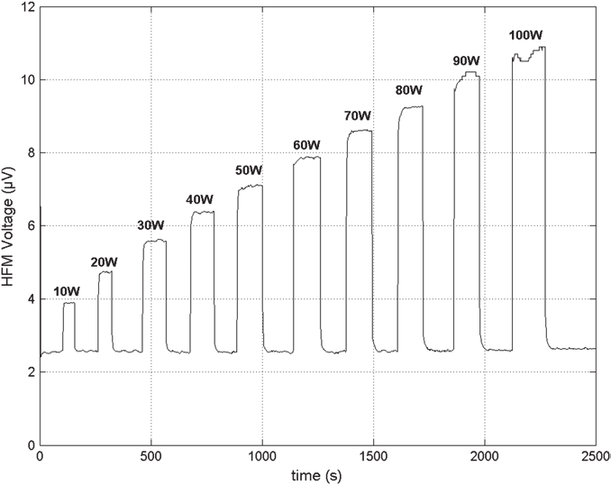
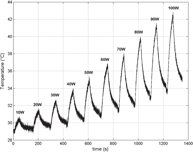
To illustrate results that can be obtained by calorimetric probes and by the HFM, typical
signals recorded in an RF argon discharge are presented in Fig. 9. Even if HFM
measurements last about 100s, it is seen on the graph that a stabiliz