Questions or comments concerning this laboratory should be directed to Prof. Charles A. Bouman, School of Electrical and Computer Engineering, Purdue University, West Lafayette IN 47907; (765) 494-0340; bouman@ecn.purdue.edu
This is the first week of a two week laboratory that covers the Discrete Fourier Transform (DFT) and Fast Fourier Transform (FFT) methods. The first week will introduce the DFT and associated sampling and windowing effects, while the second week will continue the discussion of the DFT and introduce the FFT.
In previous laboratories, we have used the Discrete-Time Fourier Transform (DTFT) extensively for analyzing signals and linear time-invariant systems.


While the DTFT is very useful analytically, it usually cannot be exactly evaluated on a computer because Equation 8.1 requires an infinite sum and Equation 8.2 requires the evaluation of an integral.
The discrete Fourier transform (DFT) is a sampled version of the DTFT, hence it is better suited for numerical evaluation on computers.


Here XN(k) is an N point DFT of x(n). Note that XN(k) is a function of a discrete integer k, where k ranges from 0 to N–1.
In the following sections, we will study the derivation of the DFT from the DTFT, and several DFT implementations. The fastest and most important implementation is known as the fast Fourier transform (FFT). The FFT algorithm is one of the cornerstones of signal processing.
The DTFT usually cannot be computed exactly because the sum in Equation 8.1 is infinite. However, the DTFT may be approximately computed by truncating the sum to a finite window. Let w(n) be a rectangular window of length N:

Then we may define a truncated signal to be

The DTFT of x tr (n) is given by:

We would like to compute  , but as with
filter design, the truncation window distorts
the desired frequency characteristics;
, but as with
filter design, the truncation window distorts
the desired frequency characteristics;
 and
and  are generally not equal.
To understand the relation between these two DTFT's,
we need to convolve in the frequency domain (as we did
in designing filters with the truncation
technique):
are generally not equal.
To understand the relation between these two DTFT's,
we need to convolve in the frequency domain (as we did
in designing filters with the truncation
technique):

where  is the DTFT of w(n).
Equation 8.8 is the periodic convolution of
is the DTFT of w(n).
Equation 8.8 is the periodic convolution of  and
and  .
Hence the true DTFT,
.
Hence the true DTFT,  ,
is smoothed via convolution with
,
is smoothed via convolution with  to produce the truncated DTFT,
  .
.
We can calculate  :
:

For ω≠0,±2π,..., we have:

Notice that the magnitude of this function is similar to sinc(ωN/2) except that it is periodic in ω with period 2π.
Equation 8.7 contains a summation over a finite number of terms. However, we can only evaluate Equation 8.7 for a finite set of frequencies, ω. We must sample in the frequency domain to compute the DTFT on a computer. We can pick any set of frequency points at which to evaluate Equation 8.7, but it is particularly useful to uniformly sample ω at N points, in the range [0,2π). If we substitute
for k=0,1,...(N–1) in Equation 8.7, we find that

In short, the DFT values result from sampling the DTFT of the truncated signal.

Download DTFT.m for the following section.
We will next investigate the effect of windowing when computing
the DFT of the signal  truncated with a window of size N=20.
In the same figure, plot the phase and magnitude
of  , using equations Equation 8.9 and
Equation 8.10.
, using equations Equation 8.9 and
Equation 8.10.
Determine an expression for  (the DTFT of the non-truncated signal).
Truncate the signal x(n) using a window of size N=20
and then use
DTFT.m
to compute  .
Make sure that the plot contains a least 512 points.
.
Make sure that the plot contains a least 512 points.
Use the command [X,w] = DTFT(x,512)
.
Plot the magnitude of  .
.
Submit the plot of the phase and magnitude of  .
.
Submit the analytical expression for  .
.
Submit the magnitude plot of  .
.
Describe the difference between  and
and  . What is the reason for this difference?
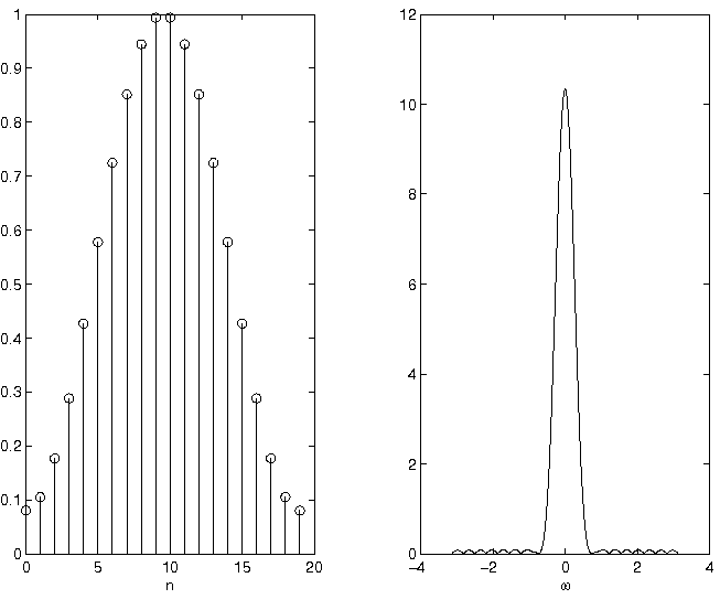
Comment on the effects of using a different window for w(n). For example, what would you expect your plots to look like if you had used a Hamming window in place of the truncation (rectangular) window? (See Figure 8.1 for a plot of a Hamming window of length 20 and its DTFT.)
We will now develop our own DFT functions to help our understanding of how the DFT comes from the DTFT. Write your own Matlab function to implement the DFT of equation Equation 8.3. Use the syntax
X = DFTsum(x)
where x
is
an N point vector containing the values x(0),⋯,x(N–1)
and X
is the corresponding DFT.
Your routine should implement the DFT exactly as specified
by Equation 8.3 using for-loops for n and k, and compute
the exponentials as they appear.
Note:
In Matlab, "j" may be computed with the command j=sqrt(-1)
. If you use  , remember not to use
j as an index in your
, remember not to use
j as an index in your for-loop.
Test your routine DFTsum by computing
XN(k) for each of the following cases:
x(n)=δ(n) for N=10.
x(n)=1 for N=10.
x(n)=ej2πn/10 for N=10.
x(n)=cos(2πn/10) for N=10.
Plot the magnitude of each of the DFT's. In addition, derive simple closed-form analytical expressions for the DFT (not the DTFT!) of each signal.
Submit a listing of your code for DFTsum.
Submit the magnitude plots.
Submit the corresponding analytical expressions.
Write a second Matlab function for computing the inverse DFT of Equation 8.4. Use the syntax
x = IDFTsum(X)
where X
is the N point vector containing the
DFT and x
is the corresponding time-domain signal.
Use IDFTsum to invert each of the DFT's computed
in the previous problem. Plot the magnitudes of the inverted DFT's,
and verify that those time-domain signals match the original ones.
Use abs(x)
to eliminate any imaginary parts
which roundoff error may produce.
Submit the listing of your code for IDFTsum.
Submit the four time-domain IDFT plots.
The DFT of Equation 8.3 can be implemented as a matrix-vector product. To see this, consider the equation
where A is an N×N matrix, and both X and x are N×1 column vectors. This matrix product is equivalent to the summation

where Akn is the matrix element in the kth row and nth column of A . By comparing Equation 8.3 and Equation 8.15 we see that for the DFT,
The –1's are in the exponent because Matlab indices start at 1, not 0. For this section, we need to:
Write a Matlab function A = DFTmatrix(N)
that returns
the NxN DFT matrix A.
Remember that the symbol * is used for matrix multiplication in Matlab, and that .' performs a simple transpose on a vector or matrix. An apostrophe without the period is a conjugate transpose.
Use the matrix A to compute the DFT of the following signals. Confirm that the results are the same as in the previous section.
x(n)=δ(n) for N=10

x(n)=ej2πn/N for N=10
Print out the matrix A for N=5.
Hand in the three magnitude plots of the DFT's.
How many multiplies are required to compute an N point DFT using the matrix method? (Consider a multiply as the multiplication of either complex or real numbers.)
As with the DFT, the inverse DFT may also be represented as a matrix-vector product.
For this section,
Write an analytical expression for the elements of the inverse DFT matrix B, using the form of Equation 8.16.
Write a Matlab function B = IDFTmatrix(N)
that returns
the NxN inverse DFT matrix B.
Compute the matrices A and B for N=5. Then compute the matrix product C=BA.
Hand in your analytical expression for the elements of B.
Print out the matrix B for N=5.
Print out the elements of C=