This is the second week of a two week laboratory that covers the Discrete Fourier Transform (DFT) and Fast Fourier Transform (FFT). The first week introduced the DFT and associated sampling and windowing effects. This laboratory will continue the discussion of the DFT and will introduce the FFT.

This section continues the analysis of the DFT started in the previous week's laboratory.

(9.1)

Shifting the Frequency Range

In this section, we will illustrate a representation for the DFT of Equation 9.1 that is a bit more intuitive. First create a Hamming window x of length N=20, using the Matlab command x = hamming(20) . Then use your Matlab function DFTsum to compute the 20 point DFT of x. Plot the magnitude of the DFT, |X₂₀(k)|, versus the index k. Remember that the DFT index k starts at 0 not 1!

INLAB REPORT

Hand in the plot of the |X₂₀(k)|. Circle the regions of the plot corresponding to low frequency components.

Our plot of the DFT has two disadvantages. First, the DFT values are plotted against k rather then the frequency ω. Second, the arrangement of frequency samples in the DFT goes from 0 to 2π rather than from –π to π, as is conventional with the DTFT. In order to plot the DFT values similar to a conventional DTFT plot, we must compute the vector of frequencies in radians per sample, and then “rotate” the plot to produce the more familiar range, –π to π.

Let's first consider the vector w of frequencies in radians per sample. Each element of w should be the frequency of the corresponding DFT sample X(k), which can be computed by

(9.2)

However, the frequencies should also lie in the range from –π to π. Therefore, if ω≥π, then it should be set to ω–2π. An easy way of making this change in Matlab 5.1 is w(w>=pi) = w(w>=pi)-2*pi .

The resulting vectors X and w are correct, but out of order. To reorder them, we must swap the first and second halves of the vectors. Fortunately, Matlab provides a function specifically for this purpose, called fftshift.

Write a Matlab function to compute samples of the DTFT and their corresponding frequencies in the range –π to π. Use the syntax

[X,w] = DTFTsamples(x)

where x is an N point vector, X is the length N vector of DTFT samples, and w is the length N vector of corresponding radial frequencies. Your function DTFTsamples should call your function DFTsum and use the Matlab function fftshift.

Use your function DTFTsamples to compute DTFT samples of the Hamming window of length N=20. Plot the magnitude of these DTFT samples versus frequency in rad/sample.

INLAB REPORT

Hand in the code for your function DTFTsamples. Also hand in the plot of the magnitude of the DTFT samples.

Zero Padding

The spacing between samples of the DTFT is determined by the number of points in the DFT. This can lead to surprising results when the number of samples is too small. In order to illustrate this effect, consider the finite-duration signal

(9.3)

In the following, you will compute the DTFT samples of x(n) using both N=50 and N=200 point DFT's. Notice that when N=200, most of the samples of x(n) will be zeros because x(n)=0 for n≥50. This technique is known as “zero padding”, and may be used to produce a finer sampling of the DTFT.

For N=50 and N=200, do the following:

1. Compute the vector x containing the values x(0),⋯,x(N–1).

2. Compute the samples of X(k) using your function DTFTsamples.

3. Plot the magnitude of the DTFT samples versus frequency in rad/sample.

INLAB REPORT

Submit your two plots of the DTFT samples for N=50 and N=200. Which plot looks more like the true DTFT? Explain why the plots look so different.

We have seen in the preceding sections that the DFT is a very computationally intensive operation. In 1965, Cooley and Tukey (1) published an algorithm that could be used to compute the DFT much more efficiently. Various forms of their algorithm, which came to be known as the fast Fourier transform (FFT), had actually been developed much earlier by other mathematicians (even dating back to Gauss). It was their paper, however, which stimulated a revolution in the field of signal processing.

It is important to keep in mind at the outset that the FFT is not a new transform. It is simply a very efficient way to compute an existing transform, namely the DFT. As we saw, a straight forward implementation of the DFT can be computationally expensive because the number of multiplies grows as the square of the input length (i.e. N² for an N point DFT). The FFT reduces this computation using two simple but important concepts. The first concept, known as divide-and-conquer, splits the problem into two smaller problems. The second concept, known as recursion, applies this divide-and-conquer method repeatedly until the problem is solved.

Consider the defining equation for the DFT and assume that N is even, so that N/2 is an integer:

(9.4)

Here we have dropped the subscript of N in the notation for X(k). We will also use the notation

to denote the N point DFT of the signal x(n).

Suppose we break the sum in Equation 9.4 into two sums, one containing all the terms for which n is even, and one containing all the terms for which n is odd:

(9.6)

We can eliminate the conditions “n even” and “n odd” in Equation 9.6 by making a change of variable in each sum. In the first sum, we replace n by 2m. Then as we sum m from 0 to N/2–1, n=2m will take on all even integer values between 0 and N–2. Similarly, in the second sum, we replace n by 2m+1. Then as we sum m from 0 to N/2–1, n=2m+1 will take on all odd integer values between 0 and N–1. Thus, we can write

(9.7)

Next we rearrange the exponent of the complex exponential in the first sum, and split and rearrange the exponent in the second sum to yield

(9.8)

Now compare the first sum in Equation 9.8 with the definition for the DFT given by Equation 9.4. They have exactly the same form if we replace N everywhere in Equation 9.4 by N/2. Thus the first sum in Equation 9.8 is an N/2 point DFT of the even-numbered data points in the original sequence. Similarly, the second sum in Equation 9.8 is an N/2 point DFT of the odd-numbered data points in the original sequence. To obtain the N point DFT of the complete sequence, we multiply the DFT of the odd-numbered data points by the complex exponential factor e^–j2πk/N, and then simply sum the two N/2 point DFTs.

To summarize, we will rewrite Equation 9.8 according to this interpretation. First, we define two new N/2 point data sequences x₀(n) and x₁(n), which contain the even and odd-numbered data points from the original N point sequence, respectively:

(9.9)

where n=0,...,N/2–1. This separation of even and odd points is called decimation in time. The N point DFT of x(n) is then given by

(9.10)

where X₀(k) and X₁(k) are the N/2 point DFT's of the even and odd points.

(9.11)

While Equation 9.10 requires less computation than the original N point DFT, it can still be further simplified. First, note that each N/2 point DFT is periodic with period N/2. This means that we need to only compute X₀(k) and X₁(k) for N/2 values of k rather than the N values shown in Equation 9.10. Furthermore, the complex exponential factor e^–j2πk/N has the property that

(9.12)

These two facts may be combined to yield a simpler expression for the N point DFT:

(9.13)

where the complex constants defined by W_N^k=e^–j2πk/N are commonly known as the twiddle factors.

Figure 9.1. 

Divide and conquer DFT of equation (13). The N-point DFT is computed using the two N/2-point DFT's X₀^(N/2)(k) and X₁^(N/2)(k) .

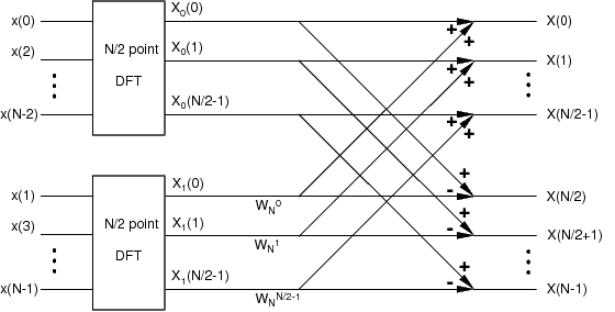
Figure 9.1 shows a graphical interpretation of Equation 9.13 which we will refer to as the “divide-and-conquer DFT”. We start on the left side with the data separated into even and odd subsets. We perform an N/2 point DFT on each subset, and then multiply the output of the odd DFT by the required twiddle factors. The first half of the output is computed by adding the two branches, while the second half is formed by subtraction. This type of flow diagram is conventionally used to describe a fast Fourier transform algorithm.

Recursive Divide and Conquer

Figure 9.2. 

Recursion of the decimation-in-time process. Now each N/2-point is calculated by combining two N/4-point DFT's.

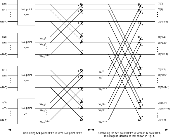
The second basic concept underlying the FFT algorithm is that of recursion. Suppose N/2 is also even. Then we may apply the same decimation-in-time idea to the computation of each of the N/2 point DFT's in

Page 1Page 2Page 3Page 4Page 5Page 6Page 7Page 8Page 9Page 10Page 11Page 12Page 13Page 14Page 15Page 16Page 17Page 18Page 19Page 20Page 21Page 22Page 23Page 24

PREV   NEXT