Questions or comments concerning this laboratory should be directed to Prof. Charles A. Bouman, School of Electrical and Computer Engineering, Purdue University, West Lafayette IN 47907; (765) 494-0340; bouman@ecn.purdue.edu
In this section, we will study the concept of a bivariate distribution. We will see that bivariate distributions characterize how two random variables are related to each other. We will also see that correlation and covariance are two simple measures of the dependencies between random variables, which can be very useful for analyzing both random variables and random processes.
Sometimes we need to account for not just one random variable, but several. In this section, we will examine the case of two random variables–the so called bivariate case–but the theory is easily generalized to accommodate more than two.
The random variables X and Y have cumulative distribution functions (CDFs) FX(x) and FY(y), also known as marginal CDFs. Since there may be an interaction between X and Y, the marginal statistics may not fully describe their behavior. Therefore we define a bivariate, or joint CDF as
If the joint CDF is sufficiently “smooth”, we can define a joint probability density function,

Conversely, the joint probability density function may be used to calculate the joint CDF:

The random variables X and Y are said to be independent if and only if their joint CDF (or PDF) is a separable function, which means
Informally, independence between random variables means that one random variable does not tell you anything about the other. As a consequence of the definition, if X and Y are independent, then the product of their expectations is the expectation of their product.
While the joint distribution contains all the information about X and Y, it can be very complex and is often difficult to calculate. In many applications, a simple measure of the dependencies of X and Y can be very useful. Three such measures are the correlation, covariance, and the correlation coefficient.
Correlation

Covariance

Correlation coefficient

If the correlation coefficient is 0, then X and Y are said to be uncorrelated. Notice that independence implies uncorrelatedness, however the converse is not true.
In the following experiment, we will examine the relationship
between the scatter plots for pairs of random samples
 and their correlation coefficient.
We will see that the correlation coefficient determines the shape of
the scatter plot.
and their correlation coefficient.
We will see that the correlation coefficient determines the shape of
the scatter plot.
Let X and Y be independent Gaussian random variables, each with mean 0 and variance 1. We will consider the correlation between X and Z, where Z is equal to the following:
Notice that since Z is a linear combination of two Gaussian random variables, Z will also be Gaussian.
Use Matlab to generate 1000 i.i.d. samples of X, denoted as X1, X2, ..., X1000. Next, generate 1000 i.i.d. samples of Y, denoted as Y1, Y2, ..., Y1000. For each of the four choices of Z, perform the following tasks:
Use Equation 11.8 to analytically calculate the correlation coefficient ρXZ between X and Z. Show all of your work. Remember that independence between X and Y implies that E[XY]=E[X]E[Y]. Also remember that X and Y are zero-mean and unit variance.
Create samples of Z using your generated samples of X and Y.
Generate a scatter plot of the ordered pair of samples  .
Do this by plotting points
.
Do this by plotting points
 ,
,  , ...,
  .
To plot points without connecting them with lines, use the '.' format, as in
.
To plot points without connecting them with lines, use the '.' format, as in plot(X,Z,'.').
Use the command subplot(2,2,n)
(n=1,2,3,4)
to plot the four cases for Z in the same figure. Be sure
to label each plot using the title command.
Empirically compute an estimate of the correlation coefficient using your samples Xi and Zi and the following formula.

Hand in your derivations of the correlation coefficient
ρXZ along with your numerical estimates of the
correlation coefficient  .
.
Why are ρXZ and  not exactly equal?
Hand in your scatter plots of  for the four cases.
Note the theoretical correlation coefficient ρXZ
on each plot.
for the four cases.
Note the theoretical correlation coefficient ρXZ
on each plot.
Explain how the scatter plots are related to ρXZ.
In this section, we will generate discrete-time random processes and then analyze their behavior using the correlation measure introduced in the previous section.
A discrete-time random process Xn is simply a sequence of random variables. So for each n, Xn is a random variable.
The autocorrelation is an important function for characterizing the behavior of random processes. If X is a wide-sense stationary (WSS) random process, the autocorrelation is defined by

Note that for a WSS random process,
the autocorrelation does not vary with n.
Also, since  , the autocorrelation
is an even function of the “lag” value m.
, the autocorrelation
is an even function of the “lag” value m.
Intuitively, the autocorrelation determines how strong a relation there is between samples separated by a lag value of m. For example, if X is a sequence of independent identically distributed (i.i.d.) random variables each with zero mean and variance σX2, then the autocorrelation is given by

We use the term white or white noise to describe this type of random process. More precisely, a random process is called white if its values Xn and Xn+m are uncorrelated for every m≠0.
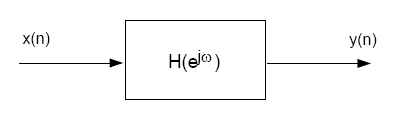
If we run a white random process Xn through an LTI filter as in Figure 11.1, the output random variables Yn may become correlated. In fact, it can be shown that the output autocorrelation rYY(m) is related to the input autocorrelation rXX(m) through the filter's impulse response h(m).
Consider a white Gaussian random process Xn with mean 0 and variance 1 as input to the following filter.
Calculate the theoretical autocorrelation of Yn using Equation 11.15 and Equation 11.16. Show all of your work.
Generate 1000 independent samples of a Gaussian random variable X with mean 0 and variance 1. Filter the samples using Equation 11.17. We will denote the filtered signal Yi, i=1,2,⋯,1000.
Draw 4 scatter plots using the form subplot(2,2,n), (n=1,2,3,4).
The first scatter plot should consist of points,  ,
(i=1,2,⋯,900). Notice that this correlates samples that are
separated by a lag of “1”.
The other 3 scatter plots should consist of the points
,
(i=1,2,⋯,900). Notice that this correlates samples that are
separated by a lag of “1”.
The other 3 scatter plots should consist of the points
 ,
,
 ,
,  , (i=1,2,⋯,900), respectively.
What can you deduce about the random process from these scatter plots?
, (i=1,2,⋯,900), respectively.
What can you deduce about the random process from these scatter plots?
For real applications, the theoretical autocorrelation may be unknown. Therefore, rYY(m) may be estimated by the sample autocorrelation, r'YY(m) defined by

where N is the number of samples of Y.
Use Matlab to calculate the sample autocorrelation of Yn using Equation 11.18. Plot both the theoretical autocorrelation rYY(m), and the sample autocorrelation r'YY(m