Questions or comments concerning this laboratory should be directed to Prof. Charles A. Bouman, School of Electrical and Computer Engineering, Purdue University, West Lafayette IN 47907; (765) 494-0340; bouman@ecn.purdue.edu
In the first and second weeks of this experiment, we introduced methods of statistically characterizing random processes. The sample autocorrelation and cross correlation are examples of “time domain” characterizations of random signals. In many applications, it can also be useful to get the frequency domain characteristics of a random process. Examples include detection of sinusoidal signals in noise, speech recognition and coding, and range estimation in radar systems.
In this week, we will introduce methods to estimate the power spectrum of a random signal given a finite number of observations. We will examine the effectiveness of the periodogram for spectrum estimation, and introduce the spectrogram to characterize a nonstationary random processes.
In this section, you will estimate the power spectrum of a stationary discrete random process. The power spectrum is defined as

There are 4 steps for calculating a power spectrum:
Select a window of length N and generate a finite sequence x(0),x(1),⋯,x(N–1).
Calculate the DTFT of the windowed sequence x(n), (n=0,1,⋯,N–1), square the magnitude of the DTFT and divide it by the length of the sequence.
Take the expectation with respect to x.
Let the length of the window go to infinity.
In real applications, we can only approximate the power spectrum. Two methods are introduced in this section. They are the periodogram and the averaged periodogram.
Click here for help on the fft command and the random command.
The periodogram is a simple and common method for estimating a power spectrum. Given a finite duration discrete random sequence x(n), (n=0,1,⋯,N–1), the periodogram is defined as

where X(ω) is the Discrete Time Fourier Transform (DTFT) of x(n).
The periodogram Pxx(ω) can be computed using the Discrete Fourier Transformation (DFT), which in turn can be efficiently computed by the Fast Fourier Transformation (FFT). If x(n) is of length N, you can compute an N-point DFT.


Using Equation 12.3 and Equation 12.4,
write a Matlab function called Pgram to calculate
the periodogram. The syntax for this function should be
[P,w] = Pgram(x)
where x is a discrete random sequence of length N. The outputs of this command are P, the samples of the periodogram, and w, the corresponding frequencies of the samples. Both P and w should be vectors of length N.
Now, let x be a Gaussian (Normal) random variable with mean 0 and
variance 1. Use Matlab function random or randn to
generate 1024 i.i.d. samples of x, and denote them as
x0, x1, ..., x1023. Then filter the samples of x with
the filter which
obeys the following difference equation

Denote the output of the filter as y0,y1,⋯,y1023.
The samples of x(n) and y(n) will be used in the following sections. Please save them.
Use your Pgram function
to estimate the power spectrum
of y(n),  .
Plot
.
Plot  vs. ωk.
Next, estimate the power spectrum of y,
 using 1/4 of the samples of y. Do this
only using samples y0, y1, ⋯, y255.
Plot
using 1/4 of the samples of y. Do this
only using samples y0, y1, ⋯, y255.
Plot  vs. ωk.
Hand in your labeled plots and your Pgram code.
Compare the two plots. The first plot uses 4 times as many samples as the second one. Is the first one a better estimation than the second one? Does the first give you a smoother estimation?
Judging from the results, when the number of samples of a discrete random variable becomes larger, will the estimated power spectrum be smoother?
The periodogram is a simple method, but it does not yield very good results. To get a better estimate of the power spectrum, we will introduce Bartlett's method, also known as the averaged periodogram. This method has three steps. Suppose we have a length-N sequence x(n).
Subdivide x(n) into K nonoverlapping segments of length M. Denote the ith segment as xi(n).

For each segment xi(n), compute its periodogram


where k=0,1,⋯,M–1 and i=0,1,⋯,K–1.
Average the periodograms over all K segments to obtain the averaged periodogram, PAxx(k),


where k=0,1,⋯,M–1.
Write a Matlab function called AvPgram to calculate
the averaged periodogram, using the above steps.
The syntax for this function should be
[P,w] = AvPgram(x, K)
where x is a discrete random sequence of length N and
the K is the number of nonoverlapping segments. The
outputs of this command are P, the samples of the averaged periodogram,
and w, the corresponding frequencies of the samples. Both
P and w should be vectors of length M where N=KM.
You may use your Pgram function.
The command A=reshape(x,M,K)
will orient length M
segments of the vector x into K columns of the matrix A.
Use your Matlab function AvPgram
to estimate the power
spectrum of y(n) which was generated in the previous section.
Use all 1024 samples of y(n), and let K=16. Plot P vs. w.
Submit your plot and your AvPgram code.
Compare the power spectrum that you estimated using the averaged periodogram with the one you calculated in the previous section using the standard periodogram. What differences do you observe? Which do you prefer?
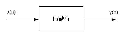
Consider a linear time-invariant system with frequency response
 , where
Sxx(ω) is the power spectrum of the input signal,
and Syy(ω) is the power spectrum of
the output signal.
It can be shown that these quantities are related by
, where
Sxx(ω) is the power spectrum of the input signal,
and Syy(ω) is the power spectrum of
the output signal.
It can be shown that these quantities are related by

In the "Periodogram" section, the sequence
y(n)
was generated by
filtering an i.i.d. Gaussian (mean=0, variance=1) sequence
x(n), using the filter in Equation 12.5.
By hand, calculate the power spectrum
Sxx(ω) of x(n),
the frequency response of the filter,
 ,
and the power spectrum
Syy(ω) of y(n).
,
and the power spectrum
Syy(ω) of y(n).
In computing
Sxx(ω),
use the fact that

Plot Syy(ω) vs. ω, and compare it with the plots from the "Periodogram" and "Averaged Periodogram" sections. What do you observe?
Hand in your plot.
Submit your analytical calculations for Sxx(ω),
 , Syy(ω).
Compare the theoretical power spectrum of Syy(ω) with the power spectrum estimated using the standard periodogram. What can you conclude?
Compare the theoretical power spectrum of Syy(ω) with the power spectrum estimated using the averaged periodogram. What can you conclude?
Download the file speech.au for this section. For help on the following Matlab topics select the corresponding link: how to load and play audio signals and specgram function.
The methods used in the last two sections can only be applied to stationary random processes. However, most signals in nature are not stationary. For a nonstationary random process, one way to analyze it is to subdivide the signal into segments (which may be overlapping) and treat each segment as a stationary process. Then we can calculate the power spectrum of each segment. This yields what we call a spectrogram.
While it is debatable whether or not a speech signal is actually random,
in many applications it is necessary to model it as being so.
In this section, you are going to use the Matlab command specgram
to calculate the spectrogram of a speech signal. Read the help for the specgram function.
Find out what the command does, and how to calculate and draw a
spectrogram.
Draw the spectrogram of the speech signal in speech.au.
When using the specgram command with no output arguments,
the absolute value of the spectrogram will be plotted.
Therefore you can use
speech=auread('speech.au');
to read the speech signal and use
specgram(speech);
to draw the spectrogram.
Hand in your spectrogram plot.
Describe the information that the spectrogram is giving you.