Questions or comments concerning this laboratory should be directed to Prof. Charles A. Bouman, School of Electrical and Computer Engineering, Purdue University, West Lafayette IN 47907; (765) 494-0340; bouman@ecn.purdue.edu
This lab presents two important concepts for working with digital signals. The first section discusses how numbers are stored in memory. Numbers may be either in fixed point or floating point format. Integers are often represented with fixed point format. Decimals, and numbers that may take on a very large range of values would use floating point. The second issue of numeric storage is quantization. All analog signals that are processed on the computer must first be quantized. We will examine the errors that arise from this operation, and determine how different levels of quantization affect a signal's quality. We will also look at two types of quantizers. The uniform quantizer is the simpler of the two. The Max quantizer, is optimal in that it minimizes the mean square error between the original and quantized signals.
There are two types of numbers that a computer can represent: integers and decimals. These two numbers are stored quite differently in memory. Integers (e.g. 27, 0, -986) are usually stored in fixed point format, while decimals (e.g. 12.34, -0.98) most often use floating point format. Most integer representations use four bytes of memory; floating point values usually require eight.
There are different conventions for encoding fixed point binary numbers because of the different ways of representing negative numbers. Three types of fixed point formats that accommodate negative integers are sign-magnitude, one's-complement, and two's-complement. In all three of these "signed" formats, the first bit denotes the sign of the number: 0 for positive, and 1 for negative. For positive numbers, the magnitude simply follows the first bit. Negative numbers are handled differently for each format.
Of course, there is also an unsigned data type which can be used when the numbers are known to be non-negative. This allows a greater range of possible numbers since a bit isn't wasted on the negative sign.
Sign-magnitude notation is the simplest way to represent negative numbers. The magnitude of the negative number follows the first bit. If an integer was stored as one byte, the range of possible numbers would be -127 to 127.
The value +27 would be represented as
0 0 0 1 1 0 1 1 .
The number -27 would represented as
1 0 0 1 1 0 1 1 .
To represent a negative number, the complement of the bits for the positive number with the same magnitude are computed. The positive number 27 in one's-complement form would be written as
0 0 0 1 1 0 1 1 ,
but the value -27 would be represented as
1 1 1 0 0 1 0 0 .
The problem with each of the above notations is that two different values represent zero. Two's-complement notation is a revision to one's-complement that solves this problem. To form negative numbers, the positive number is subtracted from a certain binary number. This number has a one in the most significant bit (MSB), followed by as many zeros as there are bits in the representation. If 27 was represented by an eight-bit integer, -27 would be represented as:
   1 0  0 0 0 0 0 0 0
   - 0  0 0 1 1 0 1 1
 =   1  1 1 0 0 1 0 1
Notice that this result is one plus the one's-complement representation for -27 (modulo-2 addition). What about the second value of 0? That representation is
1 0 0 0 0 0 0 0 .
This value equals -128 in two's-complement notation!
   1 0  0 0 0 0 0 0 0
   - 1  0 0 0 0 0 0 0
 =   1  0 0 0 0 0 0 0
The value represented here is -128; we know it is negative, because the result has a 1 in the MSB. Two's-complement is used because it can represent one extra negative value. More importantly, if the sum of a series of two's-complement numbers is within the range, overflows that occur during the summation will not affect the final answer! The range of an 8-bit two's complement integer is [-128,127].
Floating point notation is used to represent a much wider range of numbers. The tradeoff is that the resolution is variable: it decreases as the magnitude of the number increases. In the fixed point examples above, the resolution was fixed at 1. It is possible to represent decimals with fixed point notation, but for a fixed word length any increase in resolution is matched by a decrease in the range of possible values.
A floating point number, F, has two parts: a mantissa, M, and an exponent, E.
The mantissa is a signed fraction, which has a power of two in the denominator. The exponent is a signed integer, which represents the power of two that the mantissa must be multiplied by. These signed numbers may be represented with any of the three fixed-point number formats. The IEEE has a standard for floating point numbers (IEEE 754). For a 32-bit number, the first bit is the mantissa's sign. The exponent takes up the next 8 bits (1 for the sign, 7 for the quantity), and the mantissa is contained in the remaining 23 bits. The range of values for this number is (–1.18*10–38,3.40*1038).
To add two floating point numbers, the exponents must be the same. If the exponents are different, the mantissa is adjusted until the exponents match. If a very small number is added to a large one, the result may be the same as the large number! For instance, if 0.15600⋯0*230 is added to 0.62500⋯0*2–3, the second number would be converted to 0.0000⋯0*230 before addition. Since the mantissa only holds 23 binary digits, the decimal digits 625 would be lost in the conversion. In short, the second number is rounded down to zero. For multiplication, the two exponents are added and the mantissas multiplied.
Quantization is the act of rounding off the value of a signal or quantity to certain discrete levels. For example, digital scales may round off weight to the nearest gram. Analog voltage signals in a control system may be rounded off to the nearest volt before they enter a digital controller. Generally, all numbers need to be quantized before they can be represented in a computer.
Digital images are also quantized. The gray levels in a black and white photograph must be quantized in order to store an image in a computer. The “brightness" of the photo at each pixel is assigned an integer value between 0 and 255 (typically), where 0 corresponds to black, and 255 to white. Since an 8-bit number can represent 256 different values, such an image is called an “8-bit grayscale" image. An image which is quantized to just 1 bit per pixel (in other words only black and white pixels) is called a halftone image. Many printers work by placing, or not placing, a spot of colorant on the paper at each point. To accommodate this, an image must be halftoned before it is printed.
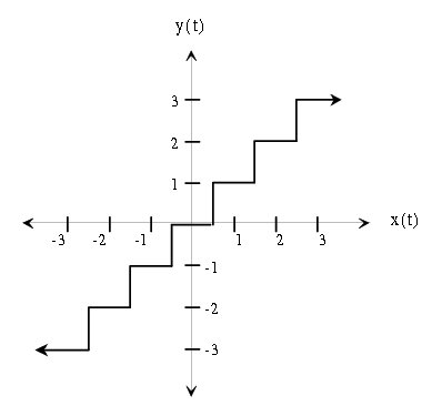
Quantization can be thought of as a functional mapping y=f(x) of a real-valued input to a discrete-valued output. An example of a quantization function is shown in Figure 13.1, where the x-axis is the input value, and the y-axis is the quantized output value.
Quantization is sometimes used for compression. As an example, suppose we have a digital image which is represented by 8 different gray levels: [0 31 63 95 159 191 223 255]. To directly store each of the image values, we need at least 8-bits for each pixel since the values range from 0 to 255. However, since the image only takes on 8 different values, we can assign a different 3-bit integer (a code) to represent each pixel: [000 001 ... 111]. Then, instead of storing the actual gray levels, we can store the 3-bit code for each pixel. A look-up table, possibly stored at the beginning of the file, would be used to decode the image. This lowers the cost of an image considerably: less hard drive space is needed, and less bandwidth is required to transmit the image (i.e. it downloads quicker). In practice, there are much more sophisticated methods of compressing images which rely on quantization.
Download the file fountainbw.tif for the following section.
The image in fountainbw.tif is an 8-bit grayscale image.
We will investigate what happens when we quantize it to fewer bits
per pixel (b/pel).
Load it into Matlab and display it using the following sequence of
commands:
y = imread('fountainbw.tif');
image(y);
colormap(gray(256));
axis('image');
The image array will initially be of type uint8, so you
will need to convert the image matrix to type
double before performing any computation.
Use the command z=double(y) for this.
There is an easy way to uniformly quantize a signal. Let

where X is the signal to be quantized, and N is the number of quantization levels. To force the data to have a uniform quantization step of Δ,
Subtract Min(X) from the data and divide the result by Δ.
Round the data to the nearest integer.
Multiply the rounded data by Δ and add Min(X) to convert the data back to its original scale.
Write a Matlab function Y = Uquant(X,N)
which will
uniformly quantize an input array X (either a vector or a matrix)
to N discrete levels.
Use this function to quantize the fountain image to
7 b/pel, 6, 5, 4, 3, 2, 1 b/pel, and observe the output images.
Remember that with b bits, we can represent N=2b gray levels.
Print hard copies of only the 7, 4, 2, and 1 b/pel images, as well as the original.
Describe the artifacts (errors) that appear in the image as the number of bits is lowered?
Note the number of b/pel at which the image quality noticeably deteriorates.
Hand in the printouts of the above four quantized images and the original.
Compare each of these four quantized images to the original.
Download the files speech.au and music.au for the following section.
If an audio signal is to be coded, either for compression or for digital transmission, it must undergo some form of quantization. Most often, a general technique known as vector quantization is employed for this task, but this technique must be tailored to the specific application so it will not be addressed here. In this exercise, we will observe the effect of uniformly quantizing the samples of two audio signals.
Down load the audio files
speech.au
and
music.au
.
Use your Uquant function to quantize each of these signals to
7, 4, 2 and 1 bits/sample.
Listen to the original and quantized signals and answer the following
questions:
For each signal, describe the change in quality as the number of b/sample is reduced?
For each signal, is there a point at which the signal quality deteriorates drastically? At what point (if any) does it become incomprehensible?
Which signal's quality deteriorates faster as the number of levels decreases?
Do you think 4 b/sample is acceptable for telephone systems? ... 2 b/sample?
Use subplot to plot in the same figure,
the four quantized speech signals over the
index range 7201:7400.
Generate a similar figure for the music signal, using the same indices.
Make sure to use orient tall before printing these out.
Hand in answers to the above questions, and the two Matlab figures.
As we have clearly observed, quantization produces errors in a signal. The most effective methods for analysis of the error turn out to be probabilistic. In order to apply these methods, however, one needs to have a clear understanding of the error signal's statistical properties. For example, can we assume that the error signal is white noise? Can we assume that it is uncorrelated with the quantized signal? As you will see in this exercise, both of these are good assumptions if the quantization intervals are small compared with sample-to-sample variations in the signal.
If the original signal is X, and the quantized signal is Y, the error signal is defined by the following:
Compute the error signal for the quantized speech for 7, 4, 2 and 1 b/sample.
When the spacing, Δ,
between quantization levels is sufficiently small,
a common statistical model for the error is a uniform
distribution from  to
to  .
Use the command
.
Use the command hist(E,20)
to generate 20-bin histograms
for each of the four error signals.
Use subplot to place the four histograms in the same figure.
Hand in the histogram figure.
How does the number of quantization levels seem to affect the shape of the distribution?
Explain why the error histograms you obtain might not be uniform?
Next we will examine correlation properties of the error signal. First compute and plot an estimate of the autocorrelation function for each of the four error signals using the following commands:
[r,lags] = xcorr(E,200,'unbiased');
plot(lags,r)
Now compute and plot an estimate of the cross-correlation function
between the quantized speech Y and each error signal E using
[c,lags] = xcorr(E,Y,200,'unbiased');
plot(lags,c)
Hand in the autocorrelation and cross-correlation estimates.
Is the autocorrelation influenced by the number of quantization levels? Do samples in the error signal appear to be correlated with each other?
Does the number of quantization levels influence the cross-correlation?
One way to measure the quality of a quantized signal is by the Power Signal-to-Noise Ratio (PSNR). This is defined by the ratio of the power in the quantized speech to power in the noise.

In this expression, the noise is the error signal E.
Generally, this means that a higher PSNR implies a less noisy signal.
From previous labs we know the power of a sampled signal, x(n), is defined by

where L is the length of x(n). Compute the PSNR for the four quantized speech signals from the previous section.
In evaluating quantization (or compression) algorithms,
a graph called a “rate-distortion curve" is often used.
This curve plots signal distortion vs. bit rate.
Here, we can measure the distortion by  , and determine
the bit rate from the number of quantization levels and sampling rate.
For example, if the sampling rate is 8000 samples/sec, and we are using
7 bits/sample, the bit rate is 56 kilobits/sec (kbps).
, and determine
the bit rate from the number of quantization levels and sampling rate.
For example, if the sampling rate is 8000 samples/sec, and we are using
7 bits/sample, the bit rate is 56 kilobits/sec (kbps).
Assuming that the speech is sampled at 8kHz, plot the
rate distortion curve using  as the measure of
distortion.
Generate this curve by computing the PSNR for 7, 6, 5,..., 1 bits/sample.
Make sure the axes of the graph
are in terms of distortion and bit rate.
as the measure of
distortion.
Generate this curve by computing the PSNR for 7, 6, 5,..., 1 bits/sample.
Make sure the axes of the graph
are in terms of distortion and bit rate.
Hand in a list of the 4 PSNR values, and the rate-distortion curve.
In this section, we will investigate a different type of quantizer which produces less noise for a fixed number of quantization levels. As an example, let's assume the input range for our signal is [-1,1], but most of the input signal takes on values between [-0.2, 0.2]. If we place more of the quantization levels closer to zero, we can lower the average error due to quantization.
A common measure of quantization error is mean squared error (noise power). The Max quantizer is designed to minimize the mean squared error for a given set of training data. We will study how the Max quantizer works, and compare its performance to that of the uniform quantizer which was used in the previous sections.
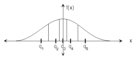
The Max quantizer determines quantization levels based on a data set's probability density function, f(x), and the number of desired levels, N. It minimizes the mean squared error between the original and quantized signals:

where qk is the kth quantization level, and xk is the lower
boundary for qk.
The error ε depends on both qk and xk.
(Note that for the Gaussian distribution,
x1=–∞, and xN+1=∞.)
To minimize ε with respect to
qk, we must take  and solve for qk:

We still need the quantization boundaries, xk.
Solving  yields:

This means that each non-infinite boundary is exactly halfway in between the two adjacent quantization levels, and that each quantization level is at the centroid of its region. Figure 13.2 shows a five-level quantizer for a Gaussian distributed signal. Note that the levels are closer together in areas of higher probability.