Questions or comments concerning this laboratory should be directed to Prof. Charles A. Bouman, School of Electrical and Computer Engineering, Purdue University, West Lafayette IN 47907; (765) 494-0340; bouman@ecn.purdue.edu
Speech is an acoustic waveform that conveys information from a speaker to a listener. Given the importance of this form of communication, it is no surprise that many applications of signal processing have been developed to manipulate speech signals. Almost all speech processing applications currently fall into three broad categories: speech recognition, speech synthesis, and speech coding.
Speech recognition may be concerned with the identification of certain words, or with the identification of the speaker. Isolated word recognition algorithms attempt to identify individual words, such as in automated telephone services. Automatic speech recognition systems attempt to recognize continuous spoken language, possibly to convert into text within a word processor. These systems often incorporate grammatical cues to increase their accuracy. Speaker identification is mostly used in security applications, as a person's voice is much like a “fingerprint”.
The objective in speech synthesis is to convert a string of text, or a sequence of words, into natural-sounding speech. One example is the Speech Plus synthesizer used by Stephen Hawking (although it unfortunately gives him an American accent). There are also similar systems which read text for the blind. Speech synthesis has also been used to aid scientists in learning about the mechanisms of human speech production, and thereby in the treatment of speech-related disorders.
Speech coding is mainly concerned with exploiting certain redundancies of the speech signal, allowing it to be represented in a compressed form. Much of the research in speech compression has been motivated by the need to conserve bandwidth in communication systems. For example, speech coding is used to reduce the bit rate in digital cellular systems.
In this lab, we will describe some elementary properties of speech signals, introduce a tool known as the short-time discrete-time Fourier Transform, and show how it can be used to form a spectrogram. We will then use the spectrogram to estimate properties of speech waveforms.
This is the first part of a two-week experiment. During the second week , we will study speech models and linear predictive coding.
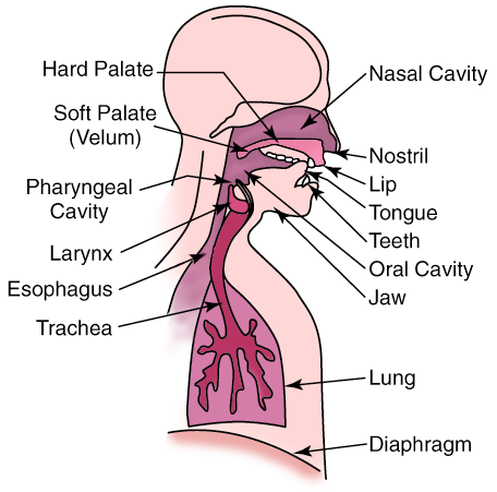
Speech consists of acoustic pressure waves created by the voluntary movements of anatomical structures in the human speech production system, shown in Figure 14.1. As the diaphragm forces air through the system, these structures are able to generate and shape a wide variety of waveforms. These waveforms can be broadly categorized into voiced and unvoiced speech.
Voiced sounds, vowels for example, are produced by forcing air through the larynx, with the tension of the vocal cords adjusted so that they vibrate in a relaxed oscillation. This produces quasi-periodic pulses of air which are acoustically filtered as they propagate through the vocal tract, and possibly through the nasal cavity. The shape of the cavities that comprise the vocal tract, known as the area function, determines the natural frequencies, or formants, which are emphasized in the speech waveform. The period of the excitation, known as the pitch period, is generally small with respect to the rate at which the vocal tract changes shape. Therefore, a segment of voiced speech covering several pitch periods will appear somewhat periodic. Average values for the pitch period are around 8 ms for male speakers, and 4 ms for female speakers.
In contrast, unvoiced speech has more of a noise-like quality. Unvoiced sounds are usually much smaller in amplitude, and oscillate much faster than voiced speech. These sounds are generally produced by turbulence, as air is forced through a constriction at some point in the vocal tract. For example, an h sound comes from a constriction at the vocal cords, and an f is generated by a constriction at the lips.
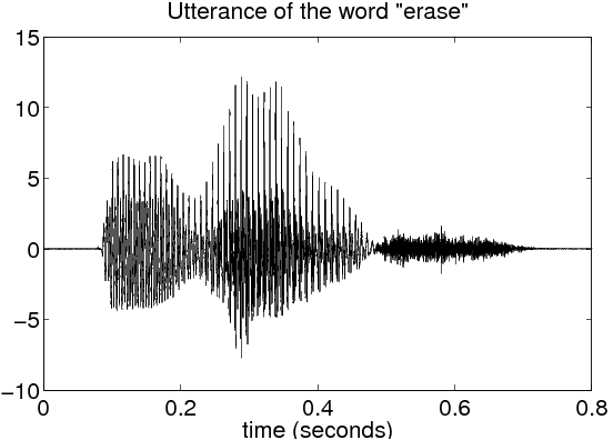
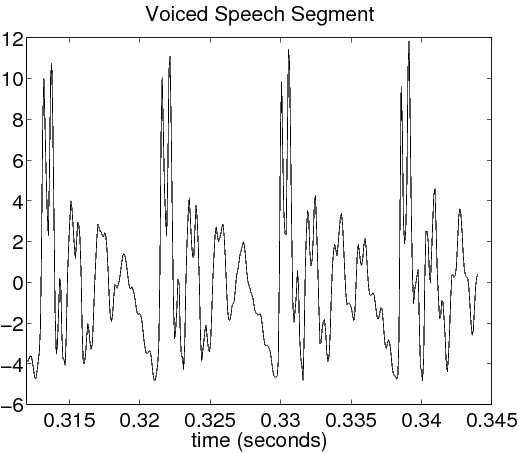
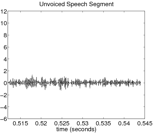
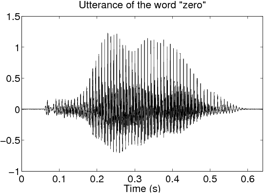
An illustrative example of voiced and unvoiced sounds contained in the word “erase” are shown in Figure 14.2. The original utterance is shown in (2.1). The voiced segment in (2.2) is a time magnification of the “a” portion of the word. Notice the highly periodic nature of this segment. The fundamental period of this waveform, which is about 8.5 ms here, is called the pitch period. The unvoiced segment in (2.3) comes from the “s” sound at the end of the word. This waveform is much more noise-like than the voiced segment, and is much smaller in magnitude.
Download the file start.au for the following sections. Click here for help on how to load and play audio signals.
For many speech processing algorithms, a very important step is to determine the type of sound that is being uttered in a given time frame. In this section, we will introduce two simple methods for discriminating between voiced and unvoiced speech.
Download the file
start.au,
and use the auread()
function to load
it into the Matlab workspace.
Do the following:
Plot (not stem) the speech signal.
Identify two segments of the signal: one segment that is voiced
and a second segment that is unvoiced (the zoom xon
command
is useful for this).
Circle the regions of the plot corresponding to these two segments
and label them as voiced or unvoiced.
Save 300 samples from the voiced segment of the speech into a Matlab vector called VoicedSig.
Save 300 samples from the unvoiced segment of the speech into a Matlab vector called UnvoicedSig.
Use the subplot()
command to plot the two signals,
VoicedSig and UnvoicedSig on a single figure.
Hand in your labeled plots. Explain how you selected your voiced and unvoiced regions.
Estimate the pitch period for the voiced segment. Keep in mind that these speech signals are sampled at 8 KHz, which means that the time between samples is 0.125 milliseconds (ms). Typical values for the pitch period are 8 ms for male speakers, and 4 ms for female speakers. Based on this, would you predict that the speaker is male, or female?
One way to categorize speech segments is to compute the average energy, or power. Recall this is defined by the following:

where L is the length of the frame x(n). Use Equation 14.1 to compute the average energy of the voiced and unvoiced segments that you plotted above. For which segment is the average energy greater?
Another method for discriminating between voiced and unvoiced segments is to determine the rate at which the waveform oscillates by counting number of zero-crossings that occur within a frame (the number of times the signal changes sign). Write a function zero_cross that will compute the number of zero-crossings that occur within a vector, and apply this to the two vectors VoicedSig and UnvoicedSig. Which segment has more zero-crossings?
Give your estimate of the pitch period for the voiced segment, and your prediction of the gender of the speaker.
For each of the two vectors,VoicedSig and UnvoicedSig, list the average energy and number of zero-crossings. Which segment has a greater average energy? Which segment has a greater zero-crossing rate?
Hand in your zero_cross function.
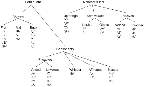
American English can be described in terms of a set of about 42 distinct sounds called phonemes, illustrated in Figure 14.3. They can be classified in many ways according to their distinguishing properties. Vowels are formed by exciting a fixed vocal tract with quasi-periodic pulses of air. Fricatives are produced by forcing air through a constriction (usually towards the mouth end of the vocal tract), causing turbulent air flow. Fricatives may be voiced or unvoiced. Plosive sounds are created by making a complete closure, typically at the frontal vocal tract, building up pressure behind the closure and abruptly releasing it. A diphthong is a gliding monosyllabic sound that starts at or near the articulatory position for one vowel, and moves toward the position of another. It can be a very insightful exercise to recite the phonemes shown in Figure 14.3, and make a note of the movements you are making to create them.
It is worth noting at this point that classifying speech sounds as voiced/unvoiced is not equivalent to the vowel/consonant distinction. Vowels and consonants are letters, whereas voiced and unvoiced refer to types of speech sounds. There are several consonants, /m/ and /n/ for example, which when spoken are actually voiced sounds.
As we have seen from previous sections, the properties of speech signals are continuously changing, but may be considered to be stationary within an appropriate time frame. If analysis is performed on a “segment-by-segment” basis, useful information about the construction of an utterance may be obtained. The average energy and zero-crossing rate, as previously discussed, are examples of short-time feature extraction in the time-domain. In this section, we will learn how to obtain short-time frequency information from generally non-stationary signals.
Download the file go.au for the following section.
A useful tool for analyzing the spectral characteristics of a non-stationary signal is the short-time discrete-time Fourier Transform, or stDTFT, which we will define by the following:

Here, x(n) is our speech signal, and w(n) is a window of length L.
Notice that if we fix m, the stDTFT is simply the DTFT of x(n)
multiplied by a shifted window. Therefore,  is a
collection of DTFTs of windowed segments of x(n).
is a
collection of DTFTs of windowed segments of x(n).
As we examined in the Digital Filter Design lab, windowing in the time domain causes an undesirable ringing in the frequency domain. This effect can be reduced by using some form of a raised cosine for the window w(n).
Write a function X = DFTwin(x,L,m,N)
that will compute the
DFT of a windowed length L segment of the vector x.
You should use a Hamming window of length L to window x.
Your window should start at the index m of the signal x.
Your DFTs should be of length N.
You may use Matlab's fft() function
to compute the DFTs.
Now we will test your DFTwin()
function.
Download the file
go.au, and load it into Matlab.
Plot the signal and locate a voiced region. Use your function to
compute a 512-point DFT of a speech segment, with a window that covers
six pitch
periods within the voiced region.
Subplot
your chosen segment and the DFT magnitude
(for ω from 0 to π) in the same figure. Label the frequency axis
in Hz, assuming a sampling frequency of 8 KHz. Remember that a radial
frequency of π corresponds to half the sampling frequency.
Hand in the code for your DFTwin() function, and your plot.
Describe the general
shape of the spectrum, and estimate the formant frequencies for the
region of voiced speech.
Download the file signal.mat for the following section.
As previously stated, the short-time DTFT is a collection of DTFTs that differ by the position of the truncating window. This may be visualized as an image, called a spectrogram. A spectrogram shows how the spectral characteristics of the signal evolve with time. A spectrogram is created by placing the DTFTs vertically in an image, allocating a different column for each time segment. The convention is usually such that frequency increases from bottom to top, and time increases from left to right. The pixel value at each point in the image is proportional to the magnitude (or squared magnitude) of the spectrum at a certain frequency at some point in time. A spectrogram may also use a “pseudo-color” mapping, which uses a variety of colors to indicate the magnitude of the frequency content, as shown in Figure 14.4.
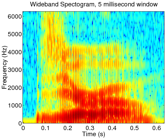
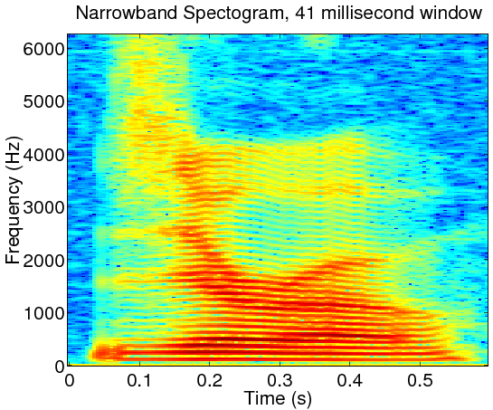
For quasi-periodic signals like speech, spectrograms are placed into two categories according to the length of the truncating window. Wideband spectrograms use a window with a length comparable to a single period. This yields high resolution in the time domain but low resolution in the frequency domain. These are usually characterized by vertical striations, which correspond to high and low energy regions within a single period of the waveform. In narrowband spectrograms, the window is made long enough to capture several periods of the waveform. Here, the resolution in time is sacrificed to give a higher resolution of the spectral content. Harmonics of the fundamental frequency of the signal are resolved, and can be seen as horizontal striations. Care should be taken to keep the window short enough, such that the signal properties stay relatively constant within the window.
Often when computing spectrograms, not every possible window shift position is used from the stDTFT, as this would result in mostly redundant information. Successive windows usually start many samples apart, which can be specified in terms of the overlap between successive windows. Criteria in deciding the amount of overlap include the length of the window, the desired resolution in time, and the rate at which the signal characteristics are changing with time.
Given this background, we would now like you to create a spectrogram
using your DFTwin()
function from the previous section.
You will do this by creating a matrix of windowed DFTs, oriented as
described above.
Your function should be of the form
A = Specgm(x,L,overlap,N)
where
x
is your input signal, L
is the window length, overlap is the number of points common to
successive windows, and N is the number of points you compute
in each DFT. Within your function, you should plot the
magnitude (in dB) of your spectrogram matrix using the command
imagesc(), and label the time and frequency axes appropriately.
Remember that frequency in a spectrogram increases along the positive y-axis, which means that the first few elements of each column of the matrix will correspond to the highest frequencies.
Your DFTwin()
function returns the DT spectrum for frequencies
between 0 and 2π. Therefore, you will only need to use the
first or second half of these DFTs.
The statement B(:,n)
references the entire nth column
of the matrix B.
In labeling the axes of the image, assume a sampling frequency of 8 KHz. Then the frequency will range from 0 to 4000 Hz.
The axis xy
command will be needed in order to
place the origin of your plot in the lower left corner.
You can get a standard gray-scale mapping (darker means greater magnitude)
by using the command colormap(1-gray)
, or a pseudo-color mapping
using the command colormap(jet)
.
For more information, see the online help for the
image
command.
Download the file
signal.mat, and load it into
Matlab. This is a raised square wave that is modulated by a sinusoid.
What would the spectrum of this signal look like?
Create both a wideband and a narrowband spectrogram using your
Specgm()
function for the signal.
For the wideband spectrogram, use a window length of 40 samples and an overlap of 20 samples.
For the narrowband spectrogram, use a window length of 320 samples, and an overlap of 60 samples.
Subplot the wideband and narrowband spectrograms, and the original signal in the same figure.
Hand in your code for Specgm() and your plots. Do you see vertical
striations in the wideband spectrogram? Similarly, do you see horizontal
striations in the narrowband spectrogram? In each case, what causes these
lines, and what does the spacing between them represent?
Download the file vowels.mat for the following section.
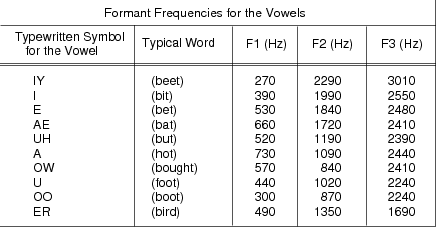
The shape of an acoustic excitation for voiced speech is similar to a triangle wave. Therefore it has many harmonics at multiples of its fundamental frequency, 1/Tp. As the excitation propagates through the vocal tract, acoustic resonances, or standing waves, cause certain harmonics to be significantly amplified. The specific wavelengths, hence the frequencies, of the resonances are determined by the shape of the cavities that comprise the vocal tract. Different vowel sounds are distinguished by unique sets of these resonances, or formant frequencies. The first three average formants for several vowels are given in Figure 14.5.
A possible technique for speech recognition would to determine a vowel utterance based on its unique set of formant frequencies. If we construct a graph that plots the second formant versus the first, we find that a particular vowel sound tends to lie within a certain region of the plane. Therefore, if we determine the first two formants, we can construct decision regions to estimate which vowel was spoken. The first two average formants for some common vowels are plotted in Figure 14.6. This diagram is