Figure 15.1. 

Discrete-Time Speech Production Model

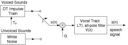
From a signal processing standpoint, it is very useful to think of speech production in terms of a model, as in Figure 15.1. The model shown is the simplest of its kind, but it includes all the principal components. The excitations for voiced and unvoiced speech are represented by an impulse train and white noise generator, respectively. The pitch of voiced speech is controlled by the spacing between impulses, T_p, and the amplitude (volume) of the excitation is controlled by the gain factor G.

As the acoustical excitation travels from its source (vocal cords, or a constriction), the shape of the vocal tract alters the spectral content of the signal. The most prominent effect is the formation of resonances, which intensifies the signal energy at certain frequencies (called formants). As we learned in the Digital Filter Design lab, the amplification of certain frequencies may be achieved with a linear filter by an appropriate placement of poles in the transfer function. This is why the filter in our speech model utilizes an all-pole LTI filter. A more accurate model might include a few zeros in the transfer function, but if the order of the filter is chosen appropriately, the all-pole model is sufficient. The primary reason for using the all-pole model is the distinct computational advantage in calculating the filter coefficients, as will be discussed shortly.

Recall that the transfer function of an all-pole filter has the form

(15.1)

where P is the order of the filter. This is an IIR filter that may be implemented with a recursive difference equation. With the input G·x(n), the speech signal s(n) may be written as

(15.2)

Keep in mind that the filter coefficients will change continuously as the shape of the vocal tract changes, but speech segments of an appropriately small length may be approximated by a time-invariant model.

This speech model is used in a variety of speech processing applications, including methods of speech recognition, speech coding for transmission, and speech synthesis. Each of these applications of the model involves dividing the speech signal into short segments, over which the filter coefficients are almost constant. For example, in speech transmission the bit rate can be significantly reduced by dividing the signal up into segments, computing and sending the model parameters for each segment (filter coefficients, gain, etc.), and re-synthesizing the signal at the receiving end, using a model similar to Figure 15.1. Most telephone systems use some form of this approach. Another example is speech recognition. Most recognition methods involve comparisons between short segments of the speech signals, and the filter coefficients of this model are often used in computing the “difference" between segments.

Download the file coeff.mat for the following section.

Download the file coeff.mat and load it into the Matlab workspace using the load command. This will load three sets of filter coefficients: A1, A2, and A3 for the vocal tract model in Equation 15.1 and Equation 15.2. Each vector contains coefficients for an all-pole filter of order 15.

We will now synthesize voiced speech segments for each of these sets of coefficients. First write a Matlab function x=exciteV(N,Np) which creates a length N excitation for voiced speech, with a pitch period of Np samples. The output vector x should contain a discrete-time impulse train with period Np (e.g. [1 0 0 ⋯ 0 1 0 0 ⋯]).

Assuming a sampling frequency of 8 kHz (0.125 ms/sample), create a 40 millisecond-long excitation with a pitch period of 8 ms, and filter it using Equation 15.2 for each set of coefficients. For this, you may use the command

s = filter(1,[1 -A],x)

where A is the row vector of filter coefficients (see Matlab's help on filter for details). Plot each of the three filtered signals. Use subplot() and orient tall to place them in the same figure.

We will now compute the frequency response of each of these filters. The frequency response may be obtained by evaluating Equation 15.1 at points along z=e^jω. Matlab will compute this with the command [H,W]=freqz(1,[1 -A],512) , where A is the vector of coefficients. Plot the magnitude of each response versus frequency in Hertz. Use subplot() and orient tall to plot them in the same figure.

The location of the peaks in the spectrum correspond to the formant frequencies. For each vowel signal, estimate the first three formants (in Hz) and list them in the figure.

Now generate the three signals again, but use an excitation which is 1-2 seconds long. Listen to the filtered signals using soundsc. Can you hear qualitative differences in the signals? Can you identify the vowel sounds?

Hand in the following:

Suppose we have a discrete-time random process whose elements have some degree of correlation. The goal of forward linear prediction is to predict the sample S_n using a linear combination of the previous P samples.

(15.3)

P is called the order of the predictor. We may represent the error of predicting S_n by a random sequence e_n.

(15.4)

An optimal set of prediction coefficients a_k for Equation 15.4 may be determined by minimizing the mean-square error . Note that since the error is generally a function of n, the prediction coefficients will also be functions of n. To simplify notation, let us first define the following column vectors.

(15.5)

(15.6)

Then,

(15.7)

The second and third terms of Equation 15.7 may be written in terms of the autocorrelation sequence r_SS(k,l).

(15.8)

(15.9)

Substituting into Equation 15.7, the mean-square error may be written as

Note that while a and r_S are vectors, and R_S is a matrix, the expression in Equation 15.10 is still a scalar quantity.

To find the optimal a_k coefficients, which we will call , we differentiate Equation 15.10 with respect to the vector a (compute the gradient), and set it equal to the zero vector.

(15.11)

Solving,

(15.12)

The vector equation in Equation 15.12 is a system of P scalar linear equations, which may be solved by inverting the matrix R_S.

Note from Equation 15.8 and Equation 15.9 that r_S and R_S are generally functions of n. However, if S_n is wide-sense stationary, the autocorrelation function is only dependent on the difference between the two indices, r_SS(k,l)=r_SS(|k–l|). Then R_S and r_S are no longer dependent on n, and may be written as follows.

(15.13)

(15.14)

Therefore, if S_n is wide-sense stationary, the optimal a_k coefficients do not depend on n. In this case, it is also important to note that R_S is a Toeplitz (constant along diagonals) and symmetric matrix, which allows Equation 15.12 to be solved efficiently using the Levinson-Durbin algorithm (see 1). This property is essential for many real-time applications of linear prediction.

An important question has yet to be addressed. The solution in Equation 15.12 to the linear prediction problem depends entirely on the autocorrelation sequence. How do we estimate the autocorrelation of a speech signal? Recall that the applications to which we are applying LPC involve dividing the speech signal up into short segments and computing the filter coefficients for each segment. Therefore we need to consider the problem of estimating the autocorrelation for a short segment of the signal. In LPC, the following "biased" autocorrelation estimate is often used.

(15.15)

Here we are assuming we have a length N segment which starts at n=0. Note that this is the single-parameter form of the autocorrelation sequence, so that the forms in Equation 15.13 and Equation 15.14 may be used for r_S and R_S.

Download the file test.mat for this exercise.

Write a function coef=mylpc(x,P) which will compute the order-P LPC coefficients for the column vector x, using the autocorrelation method (“lpc" is a built-in Matlab function, so use the name mylpc). Consider the input vector x as a speech segment, in other words do not divide it up into pieces. The output vector coef should be a column vector containing the P coefficients . In your function you should do the following:

To test your function, download the file test.mat, and load it into Matlab. This file contains two vectors: a signal x and its order-15 LPC coefficients a. Use your function to compute the order-15 LPC coefficients of x, and compare the result to the vector a.