| Classes of partial differential equations |
| Systems described by the Poisson and Laplace equation |
| Systems described by the diffusion equation |
| Greens function, convolution, and superposition |
| Green's function for the diffusion equation |
| Similarity transformation |
| Complex potential for irrotational flow |
| Solution of hyperbolic systems |
The partial differential equations that arise in transport phenomena are usually the first order conservation equations or second order PDEs that are classified as elliptic, parabolic, and hyperbolic. A system of first order conservation equations is sometimes combined as a second order hyperbolic PDE. The student is encouraged to read R. Courant, Methods of Mathematical Physics, Volume II Partial Differential Equations, 1962 for a complete discussion.
System of conservation laws. Denote the set of dependent variables (e.g., velocity, density, pressure, entropy, phase saturation, concentration) with the variable u and the set of independent variables as t and x, where x denotes the spatial coordinates. In the absence of body forces, viscosity, thermal conduction, diffusion, and dispersion, the conservation laws (accumulation plus divergence of the flux and gradient of a scalar) are of the form

This is a system of first order quasilinear hyperbolic PDEs. They can be solved by the method of characteristics. These equations arise when transport of material or energy occurs as a result of convection without diffusion.
The derivation of the equations of motion and energy using convective coordinates (Reynolds transport theorem) resulted in equations that did not have the accumulation and convective terms in the form of the conservation laws. However, by derivation of the equations with fixed coordinates (as in Bird, Stewart, and Lightfoot) or by application of the continuity equation, the momentum and energy equations can be transformed so that the accumulation and convective terms are of the form of conservation laws. Viscosity and thermal conductivity introduce second derivative terms that make the system non-conservative. This transformation is illustrated by the following relations.

For the case of inviscid, nonconducting fluid, in the absence of body forces, derive the steps to express the continuity equation, equations of motion, and energy equations as conservation law equations for mass, momentum, the sum of kinetic plus internal energy, and entropy.
For the case of isentropic, compressible flow, express continuity equation and equations of motions in terms of pressure and velocity. Transform it to a second order hyperbolic equation in the case of small perturbations.
Second order PDE. The classification of second order PDEs as elliptic, parabolic, and hyperbolic arise from a transformation of the independent variables. The classification apply to quasilinear (i.e., linear in the highest order derivatives) but we will only discuss linear equations with constant coefficients here. Numerical solutions are needed for quasilinear systems. Again let u denote the dependent variables and t, x, y, z as the independent variables. Examples of the different classes of equations are

The ρ term represents sources. When the cgs system of units is used in electrostatics and ρ is the charge density, the source is expressed as  . The factor 4π is absent with the mks or SI system of units. The parabolic PDEs are sometimes called the diffusion equation or heat equation. In the limit of steady-state conditions, the parabolic equations reduce to elliptic equations. The hyperbolic PDEs are sometimes called the wave equation. A pair of first order conservation equations can be transformed into a second order hyperbolic equation.
Convective-diffusion equation. The above equations represented convection without diffusion or diffusion without convection. When both the first and second spatial derivatives are present, the equation is called the convection-diffusion equation.

Usually a dimensionless group such as the Reynolds number, or Peclet number appears as a factor to quantify the relative contribution of convection and diffusion.
We saw earlier that an irrotational vector field can be expressed as the gradient of a scalar and if in addition the vector field is solenoidal, then the scalar potential is the solution of the Laplace equation.

Also, if the velocity field is solenoidal then the velocity can be expressed as the curl of the vector potential and the Laplacian of the vector potential is equal to the negative of the vorticity. If the flow is irrotational, then the vorticity is zero and the vector potential is a solution of the Laplace equation.

Other systems, which are solution of the Laplace equation, are steady state heat conduction in a homogenous medium without sources and in electrostatics and static magnetic fields. Also, the flow of a single-phase, incompressible fluid in a homogenous porous media has a pressure field that is a solution of the Laplace equation.
Diffusion phenomena occur with viscous flow, thermal conduction, and molecular diffusion. Heat conduction and diffusion without convection are described by the diffusion equation. Convection is always present in fluid flow but its contribution to the momentum balance is neglected for creeping (low Reynolds number) flow or cases where the velocity is perpendicular to the velocity gradient. In this case

A property of linear PDEs is that if two functions are each a solution to a PDE, then the sum of the two functions is also a solution of the PDE. This property of superposition can be used to derive solutions for general boundary, initial conditions, or distribution of sources by the process of convolution with a Green's function. The student is encouraged to read P. M. Morse and H. Feshbach, Methods of Theoretical Physics, 1953 for a discussion of Green's functions.
The Green's function is used to find the solution of an inhomogeneous differential equation and/or boundary conditions from the solution of the differential equation that is homogeneous everywhere except at one point in the space of the independent variables. (The initial condition is considered as a subset of boundary conditions here.) When the point is on the boundary, the Green's function may be used to satisfy inhomogeneous boundary conditions; when it is out in space, it may be used to satisfy the inhomogeneous PDE.
The concept of Green's solution is most easily illustrated for the solution to the Poisson equation for a distributed source ρ(x,y,z) throughout the volume. The Green's function is a solution to the homogeneous equation or the Laplace equation except at  where it is equal to the Dirac delta function. The Dirac delta function is zero everywhere except in the neighborhood of zero. It has the following property.

The Green's function for the Poisson equation in three dimensions is the solution of the following differential equation

It is a solution of the Laplace equation except at x=xo where it has a singularity, i.e., it has a point source. The solution of the Poisson equation is determined by convolution.

Suppose now that one has an elliptic problem in only two dimensions. One can either solve for the Green's function in two dimensions or just recognize that the Dirac delta function in two dimensions is just the convolution of the three-dimensional Dirac delta function with unity.

Thus the two-dimensional Green's function can be found by convolution of the three dimensional Green's function with unity.

This is a solution of the Laplace equation everywhere except at  where there is a line source of unit strength. The solution of the Poisson equation in two dimensions can be determined by convolution.

Derive the Green's function for the Poisson equation in 1-D, 2-D, and 3-D by transforming the coordinate system to cylindrical polar or spherical polar coordinate system for the 2-D and 3-D cases, respectively. Compare the results derived by convolution.
Green's functions can also be determined for inhomogeneous boundary conditions (the boundary element method) but will not be discussed here. The Green's functions discussed above have an infinite domain. Homogeneous boundary conditions of the Dirichlet type (u=0) or Neumann type (∂u/∂n=0) along a plane(s) can be determined by the method of images.
Suppose one wished to find the solution to the Poisson equation in the semi-infinite domain, y>0 with the specification of either u=0 or ∂u/∂n=0 on the boundary, y=0. Denote as u0(x,y,z) the solution to the Poisson equation for a distribution of sources in the semi-infinite domain y>0. The solutions for the Dirichlet or Neumann boundary conditions at y=0 are as follows.

The first function is an odd function of y and it vanishes at y=0. The second is an even function of y and its normal derivative vanishes at y=0.
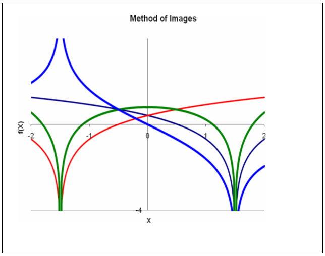
An example of the method of images to satisfy either the Dirichlet or Neumann boundary conditions is illustrated in the following figure. The black curve is the response to a line sink at x=1.5. We desire to have either the function or the derivative at x=0 to vanish. The red curve is a line sink at x=–1.5. The sum of the two functions is symmetric about x=0 and has zero derivative there. The difference is anti-symmetric about x=0 and vanishes at x=0.
Now suppose there is a second boundary that is parallel to the first, i.e. y=a that also has a Dirichlet or Neumann boundary condition. The domain of the Poisson equation is now 0<y<a. Denote as u1 the solution that satisfies the BC at y=0. A solution that satisfies the Dirichlet or Neumann boundary conditions at y=a are as follows.

This solution satisfies the solution at y=a, but no longer satisfies the solution at y=0. Denote this solution as u2 and find the solution to satisfy the BC at y=0. By continuing this operation, one obtains by induction a series solution that satisfies both boundary conditions. It may be more convenient to place the boundaries symmetric with respect to the axis in order to simplify the recursion formula.
Calculate the solution for a unit line source at the origin of the x,y plane with zero flux boundary conditions at y=+1 and y=–1. Prepare a contour plot of the solution for 0<x<5. What is the limiting solution for large x? Note: The boundary conditions are conditions on the derivative. Thus the solution is arbitrary by a constant.
If the boundary conditions for Poisson equation are the Neumann boundary conditions, there are conditions for the existence to the solution and the solution is not unique. This is illustrated as follows.

This necessary condition for the existence of a solution is equivalent to the statement that the flux leaving the system must equal the sum of sources in the system. The solution to the Poisson equation with the Neumann boundary condition is arbitrary by a constant. If a constant is added to a solution, this new solution will still satisfy the Poisson equation and the Neumann boundary condition.
We showed above how the solution to the Poisson equation with homogeneous boundary conditions could be obtained from the Green's function by convolution and method of images. Here we will obtain the Green's function for the diffusion equation for an infinite domain in one, two, or three dimensions. The Green's function is for the parabolic PDE

where the parameter a2 represents the ratio of the storage capacity and the conductivity of the system and ρ is a known distribution of sources in space and time. The infinite domain Green's function  is a solution of the following equation

The source term is an impulse in the spatial and time variables. The form of the Green's function for the infinite domain, for n dimensions, is (Morse and Feshbach, 1953)

This Green's function satisfies an important integral property that is valid for all values of n:

This expression is an expression of the conservation of heat energy. At a time to at xo, a source of heat is introduced. The heat diffuses out through the medium, but in such a fashion that the total heat energy is unchanged.
The properties of this Green's function can be more easily seen be expressing it in a standard form

The normalized function a2gn for n=3 represent the probability distribution of the location of a Brownian particle that was at xo at time to. The cumulative probability is equal to unity.
The same normalized function for n=1, corresponds to the normal or Gaussian distribution with the standard deviation given by

Observe the Green's function in one, two, and three dimensions by executing greens.m and the function, greenf.m in the diffuse subdirectory of CENG501. You may wish to use the code as a template for future assignments.
Step Response Function The infinite domain Green's function is the impulse response function in space and time. The response for a distribution of sources in space or as an arbitrary function of time can be determined by convolution. In particular the response to a constant source for τ>0 is the step response function. It has classical solutions in one and two dimensions. The unit step function or Heaviside function is the integral of the Dirac delta function.

The response function to a unit step in the source can be determined by integrating the Greens function or the impulse response function in time.

In one dimension, the step response function that has a unit flux at x=0 is (R. V. Churchill, Operational Mathematics, 1958) (note: source is  )
)

For comparison, the function that has a value of unity at x=0 (Dirichlet boundary condition) is

In two dimensions, the unit step response function for a continuous line source is (H. S. Carslaw and J. C. Jaeger, Conduction of Heat in Solids, 1959)

For large times this function can be expressed as