Couette flow
| |||
| Hele-Shaw flow | |||
Poiseuille flow
| |||
| Steady film flow down inclined plane | |||
Unsteady viscous flow
|
Chapter 2 of BSL, Transport Phenomena
One-dimensional (1-D) flow fields are flow fields that vary in only one spatial dimension in Cartesian coordinates. This excludes turbulent flows because it cannot be one-dimensional. Acoustic waves are an example of 1-D compressible flow. We will concern ourselves here with incompressible 1-D flow fields that result from axial or planar symmetry. Cartesian, 1-D incompressible flows do not have a velocity component (other than possibly a uniform translation) in the direction of the spatial dependence because of the condition of zero divergence. Thus the nonlinear convective derivative disappears from the equations of motion in Cartesian coordinates. They may not disappear with curvilinear coordinates.

We can demonstrate that this relation may not apply in curvilinear coordinates by considering an example with cylindrical polar coordinates. Suppose that the only nonzero component of velocity is in the θ direction and the only spatial dependence is on the r coordinate. The radial component of the convective derivative is non-zero due to centrifugal forces.

The flows can be classified as either forced flow resulting from the gradient of the pressure or the potential of the body force or induced flow resulting from motion of one of the bounding surfaces.
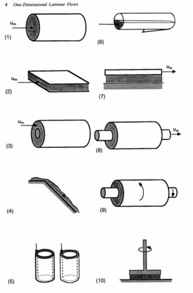
Some flow fields that result in 1-D flow are listed below and illustrated in the following figure (Churchill, 1988)
Forced flow through a round tube
Forced flow between parallel plates
Forced flow through the annulus between concentric round tubes of different diameters
Gravitational flow of a liquid film down an inclined or vertical plane
Gravitational flow of a liquid film down the inner or outer surface of a round vertical tube
Gravitational flow of a liquid through an inclined half-full round tube
Flow induced by the movement of one of a pair of parallel planes
Flow induced in a concentric annulus between round tubes by the axial movement of either the outer or the inner tube
Flow induced in a concentric annulus between round tubes by the axial rotation of either the outer or the inner tube
Flow induced in the cylindrical layer of fluid between a rotating circular disk and a parallel plane
Flow induced by the rotation of a central circular cylinder whose axis is perpendicular to parallel circular disks enclosing a thin cylindrical layer of fluid
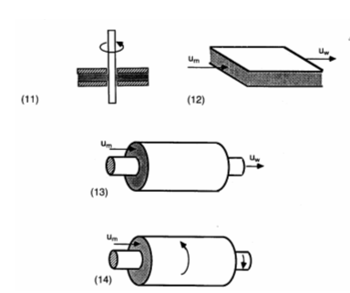
Combined forced and induced flow between parallel plates
Combined forced and induced longitudinal flow in the annulus between concentric round tubes
Combined forced and rotationally induced flow in the annulus between concentric round tubes
The flows when the fluid between two parallel surfaces are induced to flow by the motion of one surface relative to the other is called Couette flow. This is the generic shear flow that is used to illustrate Newton's law of viscosity. Pressure and body forces balance each other and at steady state the equation of motion simplify to the divergence of the viscous stress tensor or the Laplacian of velocity in the case of a Newtonian fluid.
Planar Couette flow. (case 7).

The coordinates system can be defined so that v=0 at x3=0 and the j component of velocity is non-zero at x3=L.

The velocity field is

The shear stress can be determined from Newton's law of viscosity.

Cylindrical Couette flow. The above example was the translational movement of two planes relative to each other. Couette flow is also possible in the annular gap between two concentric cylindrical surfaces (cases 8 and 9) if secondary flows do not occur due to centrifugal forces. We use cylindrical polar coordinates rather than Cartesian and assume vanishing Reynolds number. The only independent variable is the radius.

The stress profile can be calculated by integration.

The boundary conditions on velocity depend on whether the cylindrical surfaces move relative to each other as a result of rotation, axial translation, or both.

The velocity field for cylindrical Couette flow of a Newtonian fluid is .

Planer rotational Couette flow. The parallel plate viscometer has the configuration shown in case 10. The system is not strictly 1-D because the velocity of one of the surfaces is a function of radius. Also, there is a centrifugal force present near the rotating surface but is absent at the stationary surface. However, if the Reynolds number is small enough that secondary flows do not occur, then the velocity at a given value of the radius may be approximated as a function of only the z distance in the gap. The differential equations at zero Reynolds number are as follows.

Suppose the bottom surface is stationary and the top surface is rotating. Then the boundary conditions are as follows.

The stress and velocity profiles are as follows.

The stress is a function of the radius and if the fluid is non-Newtonian, the viscosity may be changing with radial position.
Forced flow between two stationary, parallel plates, case 2, is called plane-Poiseuille flow or if the flow depends on two spatial variables in the plane, it is called Hele-Shaw flow. The flow is forced by a specified flow rate or a specified pressure or gravity potential gradient. The pressure and gravitational potential can be combined into a single variable, P.

The product gh is the gravitational potential, where g is the acceleration of gravity and h is distance upward relative to some datum. The pressure, p, is also relative to a datum, which may be the datum for h.
The primary spatial dependence is in the direction normal to the plane of the plates. If there is no dependence on one spatial direction, then the flow is truly one-dimensional. However, if the velocity and pressure gradients have components in two directions in the plane of the plates, the flow is not strictly 1-D and nonlinear, inertial terms will be present in the equations of motion. The significance of these terms is quantified by the Reynolds number. If the flow is steady, and the Reynolds number negligible, the equations of motion are as follows.

Let h be the spacing between the plates and the velocity is zero at each surface.

The velocity profile for a Newtonian fluid in plane-Poiseuille flow is

The average velocity over the thickness of the plate can be determined by integrating the profile.

This equation for the average velocity can be written as a vector equation if it is recognized that the vectors have components only in the (1,2) directions.

If the flow is incompressible, the divergence of velocity is zero and the potential, P, is a solution of the Laplace equation except where sources are present. If the strength of the sources or the flux at boundaries are known, the potential, P, can be determined from the methods for the solution of the Laplace equation.
We now have the result that the average velocity vector is proportional to a potential gradient. Thus the average velocity field in a Hele-Shaw flow is irrotational. If the fluid is incompressible, the average velocity field is also solenoidal can can be expressed as the curl of a vector potential or the stream function. The average velocity field of Hele-Shaw flow is an physical analog for the irrotational, solenoidal, 2-D flow described by the complex potential. It is also a physical analog for 2-D flow of incompressible fluids through porous media by Darcy's law and was used for that purpose before numerical reservoir simulators were developed.
Poiseuille law describes laminar flow of a Newtonian fluid in a round tube (case 1). We will derive Poiseuille law for a Newtonian fluid and leave the flow of a power-law fluid as an assignment. The equation of motion for the steady, developed (from end effects) flow of a fluid in a round tube of uniform radius is as follows.

The boundary conditions are symmetry at r=0 and no slip at r=R.

From the radial component of the equations of motion, P does not depend on radial position. Since the flow is steady and fully developed, the gradient of P is a constant. The z component of the equations of motion can be integrated once to derive the stress profile and wall shear stress.

If the fluid is Newtonian, the equation of motion can be integrated once more to obtain the velocity profile and maximum velocity.

The volumetric rate of flow through the pipe can be determined by integration of the velocity profile across the cross-section of the pipe, i.e., 0<r<R and 0<θ<2π.

This relation is the Hagen-Poiseuille law. If the flow rate is specified, then the potential gradient can be expressed as a function of the flow rate and substituted into the above expressions.
The average velocity or volumetric flux can be determined by dividing the volumetric rate by the cross-sectional area.

Before one begins to believe that the Hagen-Poiseuille law is a "law" that applies under all conditions, the following is a list of assumptions are implicit in this relation (BSL, 1960).
The flow is laminar-NRe less than about 2100.
The density is constant ("incompressible flow").
The flow is independent of time ("steady state").
The fluid is Newtonian.
End effects are neglected-actually an "entrance length" (beyond the tube entrance) on the order of Le = 0.035D NRe is required for build-up to the parabolic profiles; if the section of pipe of interest includes the entrance region, a correction must be applied. The fractional correction introduced in either P or Q never exceeds Le/L if L > Le.
The fluid behaves as a continuum-this assumption is valid except for very dilute gases or very narrow capillary tubes, in which the molecular mean free path is comparable to the tube diameter ("slip flow" regime) or much greater than the tube diameter ("Knudsen flow" or "free molecule flow" regime).
There is no slip at the wall-this is an excellent assumption for pure fluids under the conditions assumed in ( f ).
Friction factor and Reynolds number. Because pressure drop in pipes is commonly used in process design, correlation expressed as friction factor versus Reynolds number are available for laminar and turbulent flow. The Hagen-Poiseuille law describes the laminar flow portion of the correlation. The correlations in the literature differ when they use different definitions for the friction factor. Correlations are usually are usually expressed in terms of the Fanning friction factor and the Darcy-Weisbach friction factor.

The Reynolds number is expressed as a ratio of inertial stress and shear stress.

Both the friction factor and the Reynolds number have as a common factor, the kinetic energy per unit volume ρum2 . This factor may be eliminated between the two equations to express the friction factor as a function of the Reynolds number.

Recall the expressions derived earlier for the wall shear stress and the average velocity for a Newtonian fluid and substitute into the above expressions.

Correlation of friction factor versus Reynolds number appear in the literature with all three definitions of the friction factor and usually without a subscript to denote which definition is being used.
Non-Newtonian fluids. The velocity profiles above were derived for a Newtonian fluid. A constitutive relation is necessary to determine the velocity profile and mean velocity for non-Newtonian fluids. We will consider the cases of a Bingham model fluid and a power-law or Ostwald-de Waele model fluid. The constitutive relations for these fluids are as follows.

The power-law model is an empirical model that is often valid over an intermediate range of shear rates. At very low and very high shear rates limiting values of viscosity are approached.
Flow in annular space between concentric cylinders as function of relative translation, rotation, potential gradient, flow or no-net flow. Assume incompressible, Newtonian fluid with small Reynolds number. The outer radius has zero velocity. Parameters:
| R2 | outer radius |
| R1 | inner radius, maybe zero |

| potential gradient, may be zero |
| Vz 1 | translation velocity of inner radius, may be zero |
| Vθ 1 | rotational velocity of inner radius |
| q | net flow rate, may be zero |
Express dimensionless velocity as a function of the dimensionless radius and dimensionless groups. Plot the following cases:
| Table of cases to plot | |||||
| Case | R1/R2 | ∂P/∂z | vz1 | vθ1 | q |
| 1 | 0 |
| |||