We already had two examples of flow in gaps that could be a thin film; Couette flow, and the steady, draining film. Here we will see that when the dimension of the gap or film thickness is small compared to other dimensions of the system, the Navier-Stokes equations simplify relatively and simple, classical solutions are possible. In Chapter 6, we saw that when the dimension of the gap or film in the x₃ direction is small and the Reynolds number is small, the equations of motion reduce to the following.

(9.1)

In the above equations, the subscript, 12, denote components in the plane of the gap or film. When the thickness is small enough, one wall of the gap or film can be treated as a plane even if it is curved with a radius of curvature that is large compared to the thickness.

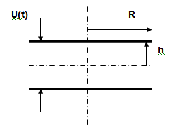
Lubrication flow with slider bearings. (Ockendon and Ockendon, 1995) Bearings function preventing contact between two moving surfaces by the flow of the lubrication fluid between the surfaces. The generic example of lubrication flow is illustrated with the slider bearing.

Figure 9.1. 

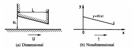
A two-dimensional bearing is shown in which the plane of y=0 moves with constant velocity U in the x-direction and the top of the bearing (the slider) is fixed. The variables are nondimensionalised with respect to U, the length L of the bearing, and a characteristic gap-width, h_o, so that the position of the slider is given in the dimensionless variables. Again, referring back to Chapter 6, the dimensionless variables for this problem may be the following.

(9.2)

Henceforth, the variables will be dimensionless with the * dropped. The boundary conditions are as follows.

(9.3)

The pressure can not suddenly equal the ambient pressure as assumed here because entrance and exit effects, but these will be neglected here. In reality, there may be a high pressure at the entrance of the bearing as a result of the liquid being scraped from the surface. The low pressure at the exit of the bearing may result in gas flowing in to equalize the pressure or cavitation may occur.

The dimensionless equations of motion and continuity equation are now as follows.

(9.4)

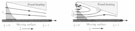
Integration of the equation of motion over the gap-thickness gives the velocity profile for a particular value of x.

(9.5)

Notice that this profile is a combination of a profile due to forced flow (pressure gradient) and that due to induced flow (movement of wall). The velocity may pass through zero somewhere in the profile if the two contributions are in opposite directions. This is illustrated in the following figure.

Figure 9.2. 

Velocity profile in slider bearing (Middleman, 1998)

Integration of the continuity equation over the thickness gives,

(9.6)

The latter integral can be expressed as follows.

(9.7)

Substituting the velocity profile into the above integral gives us the Reynolds equation for lubrication flow.

(9.8)

Integration of this equation gives,

(9.9)

A second integration gives,

(9.10)

where the constant of integration has to satisfy the boundary conditions,

(9.11)

Figure 9.3. 

Pressure profile is slider bearing (Middleman, 1998).

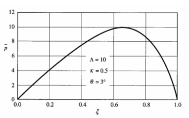
The role of the lubrication layer is to maintain a separation of the two surfaces in the presence of a load such that asperities (roughness) on the surfaces do not make contact. The load on the bearing is equal to the integral of the normal stress over the bearing surface. If the change in gap-thickness is small compared to the length, as assumed here, the normal stress is approximately equal to the pressure. If the gap-thickness is monotone decreasing, the pressure will be greater than ambient pressure inside the bearing. However, if the gap-thickness in monotone increasing, the pressure will be less than ambient in the bearing and it will have no load bearing capacity. If the gap-thickness is not monotone, then the pressure may be greater than ambient in some places and less than ambient in other places. If the bearing is designed to be load bearing, then a long section of decreasing gap-thickness and a short section of increasing thickness is desired. If the bearing is designed to be a scraper as piston rings then both sections of changing thickness will be short as to limit the amount of liquid passing through the gap. Gas entering the low-pressure region at the exit of the bearing surface prevents bearing surface contact from negative pressures.

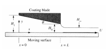
The analysis for the slider bearing can also be used to design an apparatus for depositing a uniform coating of a liquid on a substrate.

Figure 9.4. 

Coating flow (Middleman, 1998)

Squeeze films. When two objects approach each other in a fluid their relative velocity is slowed as the resistance increases for the fluid leaving the gap. Here the relative velocity of the surface is in the normal direction rather than in the parallel direction as in the case of the slider bearing. This type of flow is important in the coalescence of emulsion droplets or foam bubbles. In the case of coalescence, hydrodynamics govern the dynamics of the approach of the surfaces to each other until the thinning is accelerated or retarded by surface forces (i.e., disjoining pressure).

We will derive the classical Reynolds drainage of a liquid between two parallel disks of radius R approaching each other. The configuration of the system is shown below.

Figure 9.5. 

Schematic of film drainage between parallel disks

The system is symmetrical about its axis and the mid-plane. The thickness, h, is one-half of the distance between the disks and the velocity of each disk, U, is one-half of the approach velocity of the two disks. This nomenclature may be awkward but with this nomenclature, the solution also applies to the thinning of a liquid film between a solid surface and a gas bubble having zero shear stress at the interface. The velocity of approach of the disks may not be constant but rather the force pressing the disks together may be constant. Because of the symmetry, we will analyze the upper half-space with cylindrical polar coordinates. The system is axisymmetrical so the independent variables are r, z, t. The equations of motion and continuity equation in cylindrical polar coordinates are

(9.12)

The boundary conditions are

(9.13)

The partial differential equations do not have an explicit dependence on time as time only enters thorough the boundary conditions. Thus the variables will be made dimensionless with respect to the time dependent boundary conditions for the purpose of solving the PDE.

(9.14)

The dimensionless equations and boundary conditions with the * dropped are now

(9.15)

Integration of v_r with respect to z in the equation of motion and applying the boundary conditions results in the velocity profile across the film thickness.

(9.16)

Integration of the continuity equation over the film thickness gives,

(9.17)

The velocity profile across the thickness is substituted into the above equation and the integration preformed.

(9.18)

Integration and application of the boundary conditions give

(9.19)

The pressure and radius can now be converted to dimensional variables so we can see the dependence of the parameters.

(9.20)

The pressure distribution has a maximum at the center of the disk and decreases to zero at the outer radius of the disk. The pressure integrated over the area of the disk gives the force required to bring the disks together, each disk with a velocity U, when each disk is a distance h from the midplane.

(9.21)

This expression can be turned around to express the velocity of each disk approaching each other when a force F is applied.

(9.22)

This result is the classical Reynolds (1886) velocity for the thinning of two parallel disks.

If the applied force is constant, the above equation can be integrated to determine the time it takes to thin down from some initial thickness, h_i.

(9.23)

It the initial thickness is large but unknown, then it can be assumed to be infinity with only a small error in the time to thin down to a small thickness. An explicit expression for the time to thin from infinite thickness to a thickness h is

(9.24)

From this expression, we see that it will take an infinite time to thin to zero thickness. In reality, as the film becomes very thin, surface forces (disjoining pressure) will become important in accelerating or retarding the rate of thinning. If the surfaces are solid surfaces, contact will be made at high points (roughness) and the contact stresses may limit the thinning.

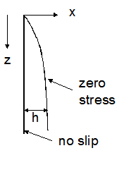
Transient Drainage of a Vertical Film Earlier we treated the steady film flow along an inclined plane. Here we will consider the transient drainage of a film that has zero flux at the upstream boundary. This corresponds to the transient behavior immediately after the flow if liquid is shut off in the problem of the steady flow along an incline plane. We will treat the wall as if it was vertical. If it is inclined from the vertical, the acceleration of gravity in the solution will need to be multiplied by the cosine of the angle from the vertical. It is assumed that the film is thin enough for the Reynolds number to be negligible and there are no ripples. Also, it is assumed that the thickness is large enough that surface forces (disjoining pressure) are negligible. The fluid in the film is assumed to be incompressible and Newtonian and the surrounding fluid is assumed to have zero density and viscosity. The surface tension and surface viscosity are neglected. The initial thickness of the film is assumed to be a constant value, h_i. Let z be the coordinate in the direction of the film flow and x the direction perpendicular to the wall. The equations of motion and continuity equation for thin films, discussed in Chapter 6 have several terms that can be neglected. The resulting equations and boundary conditions follows.

(9.25)

Figure 9.6. 

The first equation states that there is zero potential gradient over the thickness of the film. Because the surrounding fluid has zero density and the surface tension is neglected, the pressure in the film is equal to that of the surrounding fluid. Thus,

(9.26)

The velocity profile across the thickness of the film can be determined by integrating the second equation.

(9.27)

The flux or flow rate per unit width of the film can be determined by integrating the velocity profile over the thickness of the film.

(9.28)

The continuity equation can be integrated over the thickness of the film.

(9.29)

The derivative can be taken outside of the integral with the addition of another term that cancels the term in the previous equation.

(9.30)

Thus the differential equation for the film thickness is

(9.31)

This is a first order, hyperbolic partial differential equation with constant initial and boundary conditions. Time and distance can be combined into a single similarity variable. The trajectories of constant values of the dependent variable can be calculated from the PDE.

(9.32)

Since the origin of all changes in thickness occur at the origin, the equation can be integrated as straight-line trajectories for each value of thickness between zero and the initial condition.

(9.33)

This is the classical solution for transient film drainage. Thick films initially drain very rapidly but the rate of drainage slows as the film thins.

Notice that where the thickness has thinned below the initial thickness, the thickness is independent of the value of the initial thickness. Also, notice that the solution does not have a characteristic time, length, or thickness. This suggests that the thickness, time and distance are self-similar. In fact these variables can be combined into a single variable.

(9.34)

The thickness normalized with respect to the initial thickness can be expressed as a function of a single similarity variable or if a system length is specified, it can be expressed as a function of the dimensionless distance and time.

One may be interested in the volume of liquid that remains on a vertical wall of length L after the film is everywhere less than the initial thickness. This can be determined by integrating the film thickness profile over the length of the wall.

(9.35)

This expression shows that the amount of liquid remaining on a vertical wall is inversely proportional to the square root of time. This solution is valid only after the film has everywhere thinned below the initial thickness.

Transient drainage of vertical film.

The flow of an ideal fluid (inviscid and incompressible) in two dimensions can be calculated for many configurations through the use of potential flow and complex variables. At a solid boundary, the ideal fluid has zero flux (the normal component of velocity is equal to that of the solid) but the tangential velocity may not be equal to that of the solid. Real fluids have a finite viscosity and (with only a few exceptions) the tangential component of velocity is equal to that of the solid, i.e., the boundary condition of no-slip. In many cases, the "external flow" sufficiently far from a solid body can be modeled as that of an ideal fluid and the effect of finite viscosity effects the flow only near the surface of the body (and downstream of the body). These situations can be treated by application of the boundary layer theory.

The underlying assumption in the boundary layer theory is that there is a very thin layer near the body where the gradient of the tangential velocity is very large due to the action of viscosity and the no-slip boundary condition. Elsewhere the effect of viscosity is assumed to be unimportant and can be modeled as inviscid or potential flow.

The continuity equation and equations of motion were specialized in Chapter 6 with the assumption that the boundary layer thickness,δ , is small compared to the characteristic dimension of the body, L, i.e., δ/L<<1. The equations (known as Prandtl's boundary layer equations) and boundary conditions are recalled here.

Figure 9.7. 

Boundary layer flow along a wall (Schlichting, 1960)

(9.36)

(9.37)

The remaining terms in the equation of motion and continuity equation are of similar magnitude if