2013/05/17 13:45:40 -0500
Consider a stationary ergodic source, where we no longer assume that it is parametric. We need to define notions of probability that fit the universal framework. For this, we study Kac's lemma 5.
We have a stationary source,  ,
,
 .
Define Nr as the number of shifts forward of a window of length ℓ until we see z again;
this is called recurrence time. Define
.
Define Nr as the number of shifts forward of a window of length ℓ until we see z again;
this is called recurrence time. Define

e.g., Y0=1, then Nr is the smallest positive number for which Yk=1. Note that  is a binary stationary ergodic source. Define
  .
Then the average recurrence time can be computed,
.
Then the average recurrence time can be computed,  .
We can now present Kac's lemma.
.
We can now present Kac's lemma.
Lemma 3 5 and E[Nr =μ| X0–ℓ+1 = z]=
 .
.
Let  . Because z just appeared, then its probability is positive. We will prove that
  .
.
Define  , and
, and  . Then
  . We claim that
  . This can be shown formally, but is easily seen by realizing that if z appears at any time n (say, positive) then it must appear at some negative time n with probability 1, because its probability is positive.
Therefore, we have

Therefore,  We conclude the proof by noting that Pr(A)=0.
Let us now develop a universal coding technique for stationary sources. Recall  . The asymptotic equipartition property (AEP) of information
theory 1 gives
. The asymptotic equipartition property (AEP) of information
theory 1 gives

where limℓ→∞ϵ(δ,ℓ)=0. Define in this context a typical set T(δ,ℓ) that satisfies

For a typical sequence z,  . Then

Consider our situation, we have a source with memory of length n and want to transmit X1ℓ.
Choose  .
.
For z=X1ℓ, find the value of Nr if it appears in memory.
If it appears, then transmit a 0 flag bit followed by the value of Nr.
Else transmit a 1 followed by the uncompressed z.
Transmitting z via Nr requires  bits, and so
the expected coding length is
bits, and so
the expected coding length is

After we normalize by ℓ, the per symbol length converges to  .
.
Note that this analysis assumes that the entropy Hℓ for a block of ℓ symbols is known. If not, then we can have several sets that are each adjusted for some different entropy level.
Coding of an index also appears in other information theoretic problems such as indexing a coset in distributed source coding and a codeword in lossy coding. What are good ways to encode the index?
If the index n lies in the range n∈{1,...,N} and N is known, then we can encode the index using ⌈log(N)⌉ bits. However, sometimes the index can be unbounded, or there could be an (unknown) distribution that biases us strongly toward smaller indices. Therefore, we are interested in a universal encoding of the integers such that each n is encoded using roughly log(n) bits.
To do so, we outline an approach by Elias 2. Let n be a natural number, and let b(n)be the binary form for n. For example, b(0)=0,b(1)=1,b(2)=10,b(3)=11, and so on. Another challenge is that the length of this representation, |b(n)|, is unknown. Let u(k)=0k–11, for example u(4)=0001. We can now define e(n)=u(|b(|b(n)|)|)b(|b(n)|)b(n). For example, for n=5, we have b(n)=101. Therefore, |b(n)|=3,b(|b(n)|)=11,|b(|b(n)|)|=2,u(|b(|b(n)|)|)=01, and e(n)=0111101. We note in passing that the first 2 bits of e(n) describe the length of b(|b(n)|), which is 2, the middle 2 bits describe b(|b(n)|), which is 3, and the last 3 bits describe b(n), giving the actual number 5. It is easily seen that

Having described an efficient way to encode an index, in particular a large one, we can employ this technique in sliding window coding as developed by Wyner and Ziv 7.
Take a fixed window of length nw and a source that generates characters.
Define the history as x1nw, this is the portion of the data x that we
have already processed and thus know.
Our goal is to encode the phrase  ,
where L1 is not fixed.
The length L1 is chosen such that there exists
,
where L1 is not fixed.
The length L1 is chosen such that there exists

for some  .
For example, if x=abcbababc and we have processed the first 5
symbols abcba, then L1=3 and m1=1, where abcba is the history
and we begin encoding after that part.
.
For example, if x=abcbababc and we have processed the first 5
symbols abcba, then L1=3 and m1=1, where abcba is the history
and we begin encoding after that part.
The actual encoding of the phrase y1 sends  bits,
where
bits,
where

First we encode L1; then either the index m into history is encoded or y1 is encoded uncompressed; finally, the first L1 characters x1L1 are removed from the history database, and y1 is appended to its end. The latter process gives this algorithm a sliding window flavor.
This rather simple algorithm turns out to be asymptotically optimal in the limit of large nw.
That is, it achieves the entropy rate.
To see this, let us compute the compression factor.
Consider x1N where
N>>nw,
 ,
N=∑Ci=1|yi|,
and |yi|=L1,
where C is the number of phrases required to encode x1N.
The number of bits
,
N=∑Ci=1|yi|,
and |yi|=L1,
where C is the number of phrases required to encode x1N.
The number of bits  needed to encoded x1N using the
sliding window algorithm is
needed to encoded x1N using the
sliding window algorithm is

Therefore, the compression factor  satisfies

Claim 3 7
As limnw→∞ and limN→∞, the compression factor
 converges to the entropy rate H.
A direct proof is complicated, because the location of phrases is a random variable, making a detailed analysis complicated. Let us try to simplify the problem.
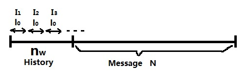
Take l0 that divides nw+N to create  intervals,
where
intervals,
where  , which is related to the window
size in the algorithm from Chapter 7.
This partition into blocks appears in Figure 7.1.
Denote by wl0(x)>0 the smallest value for which
, which is related to the window
size in the algorithm from Chapter 7.
This partition into blocks appears in Figure 7.1.
Denote by wl0(x)>0 the smallest value for which
 .
Using Kac's lemma 5,
.
Using Kac's lemma 5,

Claim 4 7 We have the following convergence as l increases,

Because of the AEP 1,

Therefore, for a typical input  .
.
Recall that the interval length is  and so the probability
that an interval cannot be found in the history is
and so the probability
that an interval cannot be found in the history is

For a long enough interval, this probability goes to zero.
There are many Ziv-Lempel style parsing algorithms 8, 9, 7,
and each of the variants
has different details, but the key idea is to find the longest match
in a window of length nw.
The length of the match is L, where we remind the reader
that  .
.
Now, encoding L requires  bits, and so the per-symbol
compression ratio is
bits, and so the per-symbol
compression ratio is  , which in the limit of large
nw approaches the entropy rate H.
, which in the limit of large
nw approaches the entropy rate H.
However, the encoding of L must also desribe its length, and often
the symbol that follows the match. These require length
 , and the normalized (per-symbol) cost is

Therefore, the redundancy of Ziv-Lempel style compression algorithms is proportional to