For i.i.d. sources, , which means that the divergence increases linearly with n. Not only does the divergence increase, but it does so by a constant per symbol. Therefore, based on typical sequence concepts that we have seen, for an xⁿ generated by P₁, its probability under P₂ vanishes. However, we can construct a distribution Q whose divergence with both P₁ abd P₂ is small,

(3.1)

We now have for P₁,

(3.2)

On the other hand, Equation 2.8, and so

(3.3)

By symmetry, we see that Q is also close to P₂ in the divergence sense.

Intuitively, it might seem peculiar that Q is close to both P₁ and P₂ but they are far away from each other (in divergence terms). This intuition stems from the triangle inequality, which holds for all metrics. The contradiction is resolved by realizing that the divergence is not a metric, and it does not satisfy the triangle inequality.

Note also that for two i.i.d. distributions P₁ and P₂, the divergence

(3.4)

is linear in n. If Q were i.i.d., then must also be linear in n. But the divergence is not increasing linearly in n, it is upper bounded by 1. Therefore, we conclude that Q(·) is not an i.i.d. distribution. Instead, Q is a distribution that contains memory, and there is dependence in Q between collections of different symbols of x in the sense that they are either all drawn from P₁ or all drawn from P₂. To take this one step further, consider K sources with

(3.5)

then in an analogous manner to before it can be shown that

(3.6)

Sources with memory: Instead of the memoryless (i.i.d.) source,

(3.7)

let us now put forward a statistical model with memory,

(3.8)

Stationary source: To understand the notion of a stationary source, consider an infinite stream of symbols, ...,x_–1,x₀,x₁,.... A complete probabilistic description of a stationary distribution is given by the collection of all marginal distribution of the following form for all t and n,

(3.9)

For a stationary source, this distribution is independent of t.

Entropy rate: We have defined the first order entropy of an i.i.d. random variable Equation 2.6, and let us discuss more advanced concepts for sources with memory. Such definitions appear in many standard textbooks, for example that by Gallager 1.

The entropy rate also satisfies .

Theorem 3 For a stationary source with bounded first order entropy, H₁(x)<∞, the following hold.

Proof. Part (1):

(3.13)

Part (2):

(3.14)

Part (3): This comes from the fist equality in the proof of (2), because we have the average of a monotonely non-increasing sequence.

Part (4): Both sequences are monotone non-increasing (parts (1) and (3)) and bounded below (by zero). Therefore, they both have a limit. Denote and .

Owing to part(2), . Therefore, it suffices to prove .

(3.15)

Now fix n and take the limit for large m. The inequality appears, which proves that both limits are equal.

Coding theorem: Theorem 3 yields for fixed to variable length coding that for a stationary source, there exists a lossless code such that the compression rate ρ_n obeys,

(3.16)

This can be proved, for example, by choosing , which is a Shannon code. As n is increased, the compression rate ρ_n converges to the entropy rate.

We also have a converse theorem for lossless coding of stationary sources. That is, .

3.1. Stationary Ergodic Sources

Consider the sequence . Let x^'=S_x denote a step ∀n∈Z, x_n^'=x_n+1, where S_xⁱ takes i steps. Let f_k(x) be a function that operates on coordinates . An ergodic source has the property that empirical averages converge to statistical averages,

(3.17)

In block codes we want

(3.18)

We will be content with convergence in probability, and a.s. convergence is better.

Theorem 4 Let X be a stationary ergodic source with H₁(x)<∞, then for every ϵ>0,δ>0, there exists n₀(δ,ϵ) such that ∀n≥n₀(δ,ϵ),

(3.19)

where .

The proof of this result is quite lengthy. We discussed it in detail, but skip it here.

Theorem 4 is called the ergodic theorem of information theory or the ergodic theorem of entropy. Shannon (48') proved convergence in probability for stationary ergodic Markov sources. McMillan (53') proved L¹ convergence for stationary ergodic sources. Brieman (57'/60') proved convergence with probability 1 for stationary ergodic sources.

3.2. Parametric Models of Information Sources

In this section, we will discuss several parametric models and see what their entropy rate is.

Memoryless sources: We have seen for memoryless sources,

(3.20)

where there are r–1 parameters in total,

(3.21) θ = { p ( a ) , a = 1 , 2 , . . . , r – 1 } ,

the parameters are denoted by θ, and α={1,2,...,r} is the alphabet.

Markov sources: The distribution of a Markov source is defined as

(3.22)

where n≥k. We must define initial probabilities and transition probabilities, . There are r^k–1 initial probabilities and (r–1)r^k transition probabilities, giving a total of r^k+1–1 parameters. Note that

(3.23)

Therefore, the space of Markov sources covers the stationary ergodic sources in the limit of large k.

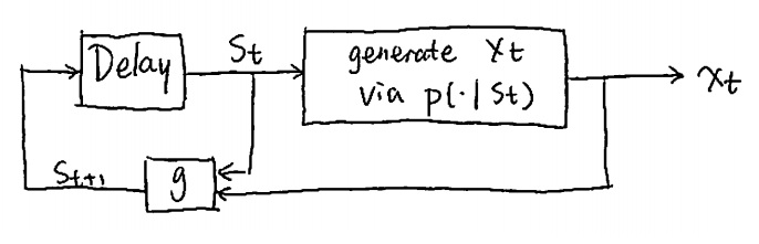
Unifilar sources: For unifilar sources, it is possible to reconstruct the set of states that a source went through by looking at the output sequence. In the Markov case we have , but in general it may be more complicated to determine the state.

To put us on a concrete basis for analysis of unifilar sources, consider a source with M states, S={1,2,...,M}, and an alphabet α={1,2,...,r}. In each time step, the source outputs a symbol and moves to a new state. Denote the output sequence by x=x₁x₂⋯x_n, and the state sequence by s=s₁s₂⋯s_n, where s_i∈S and x_i∈α. Denote also

(3.24)

This is a first-order time-homogeneous Markov source. The probability that the next symbol is a follows,

(3.25)

There exists a deterministic function,

(3.26)

this is called the next state function. Given that we start at some state S₁=s₁, the probability for the sequence of states s₁,...,s_n is given by

(3.27)

Note the relation

(3.28)

To summarize, unifilar sources can be described by a state machine style of diagram as illustrated in Figure 3.1.

Figure 3.1. 

State machine for selecting the state of a unifilar source.

Given that an initial state was fixed, a unifilar source with M states and an alphabet of size r can be expressed with M(r–1) parameters. If the initial state is a random variable, then there are M–1 parameters that define probabilities for the initial state, giving M(r–1)+M–1=Mr–1 parameters in total. In the Markov case, we have M=r^k, it is a special type of unifilar source.

Example 3.1. 

For the unifilar source that appears in Figure 3.2, the states can be discerned from the output sequence. Let us follow up on this example while discussing more properties of unifilar sources.

Page 1Page 2Page 3Page 4Page 5Page 6Page 7Page 8Page 9Page 10Page 11Page 12Page 13Page 14Page 15Page 16

PREV   NEXT