2013/05/21 14:35:15 -0500
Recall that a context tree source is similar to a Markov source, where the number of states is greatly reduced. Let T be the set of leaves of a context tree source, then the redundancy is

where |T| is the number of leaves, and we have  instead of log(n), because each state generated
  symbols, on average.
In contrast, the redundancy for a Markov representation of the tree source T is much larger.
Therefore, tree sources are greatly preferable in practice, they offer a significant reduction
in redundancy.
symbols, on average.
In contrast, the redundancy for a Markov representation of the tree source T is much larger.
Therefore, tree sources are greatly preferable in practice, they offer a significant reduction
in redundancy.
How can we compress universally over the parametric class of tree sources? Suppose that we
knew T, that is we knew the set of leaves. Then we could process x sequentially, where
for each xi we can determine what state its context is in, that is the unique suffix of
x1i–1 that belongs to the set of leaf labels in T. Having determined that we are
in some state s,  can be computed by examining all
previous times that we were in state s and computing the probability with the
Krichevsky-Trofimov approach based on the number of times that the following symbol
(after s) was 0 or 1. In fact, we can store symbol counts nx(s,0) and nx(s,1) for
all s∈T, update them sequentially as we process x, and compute
can be computed by examining all
previous times that we were in state s and computing the probability with the
Krichevsky-Trofimov approach based on the number of times that the following symbol
(after s) was 0 or 1. In fact, we can store symbol counts nx(s,0) and nx(s,1) for
all s∈T, update them sequentially as we process x, and compute
 efficiently. (The actual translation to bits is performed with an
arithmetic encoder.)
efficiently. (The actual translation to bits is performed with an
arithmetic encoder.)
While promising, this approach above requires to know T. How do we compute the optimal T* from the data?
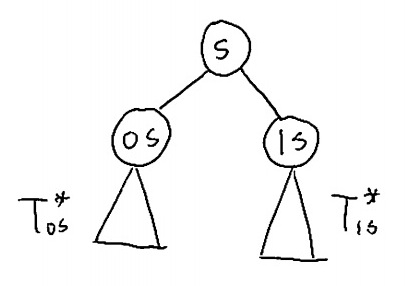
Semi-predictive coding: The semi-predictive approach to encoding for context tree sources 6 is to scan the data twice, where in the first scan we estimate T* and in the second scan we encode x from T*, as described above. Let us describe a procedure for computing the optimal T* among tree sources whose depth is bounded by D. This procedure is visualized in Figure 5.1. As suggested above, we count nx(s,a), the number of times that each possible symbol appeared in context s, for all s∈αD,a∈α. Having computed all the symbol counts, we process the depth-D tree in a bottom-top fashion, from the leaves to the root, where for each internal node s of the tree (that is, s∈αd where d<D), we track Ts*, the optimal tree structure rooted at s to encode symbols whose context ends with s, and MDL(s) the minimum description lengths (MDL) required for encoding these symbols.
Without loss of generality, consider the simple case of a binary alphabet α={0,1}. When processing s we have already computed the symbol counts nx(0s,0) and nx(0s,1), nx(1s,0), nx(1s,1), the optimal trees T*0s and T*1s, and the minimum description lengths (MDL) MDL(0s) and MDL(1S). We have two options for state s.
KeepT*0S and T*1S. The coding length required to do so is MDL(0S)+MDL(1S)+1, where the extra bit is spent to describe the structure of the maximizing tree.
Merge both states (this is also called tree pruning). The symbol counts will be nx(s,α)=nx(0s,α)+nx(1s,α),α∈{0,1}, and the coding length will be

where KT(·,·) is the Krichevsky-Trofimov length 4, and we again included an extra bit for the structure of the tree.
We note in past that there is no need to spend a bit to encode leaves of depth D. To see this, consider a procedure for encoding the structure of a tree:
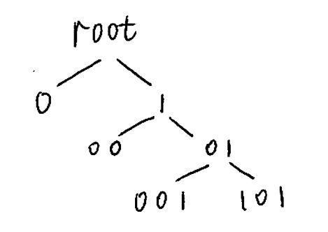
Consider the tree sourced depicted in Figure 5.2. In order to encode the structure of this tree, we will utilize the following procedure. (Such a procedure has appeared, for example, in 8.)
Start from root. [procedure(root)]
1. If node S is of depth D (maximum), then return.
2. If node S is internal node, then {
encode 0
procedure(0S)
procedure(1S)
} else encode 1.
3. return.
Let us now simulate the procedure, the procedure will traverse through the following states of the tree in Figure 5.2 while outputting the corresponding bits.
| Source | root | 0 | 1 | 01 | 001 | 101 | 11 |
| Encoded symbol | 0 | 1 | 0 | 0 | 1 |
Returning to tree pruning, following Example 5.1
we see that we must initialize
 for s of full depth |s|=D
without the extra bit.
for s of full depth |s|=D
without the extra bit.
At the end of the pruning procedure, T*{} the maximizing tree for the root, will be the optimal tree for universal coding.
The Burrows Wheeler transform (BWT) was proposed by Burrows and Wheeler in 1994 2 (see also the analysis by Effros et al. 3 and references therein). It is an invertible permutation sort that sorts symbols according to their contexts. That way, the symbols that were generated by the same state of the context tree are grouped together, which as we will see is advantageous.
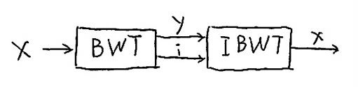
To compute the BWT, we first compute all cyclical shifts of the input x. Next, we sort the cyclical shifts. The output of the BWT consists of y, the last column of the matrix of sorted shifts, and i the index of the original version. We illustrate with an example.
Consider the input x=banana. First, we compute the cyclic shifts and their sorts.
| All Shifts | Sorted |
| banana | abanan |
| abanan | anaban |
| nabana | ananab |
| anaban | banana |
| nanaba | nabana |
| ananab | nanaba |
The output of the BWT consists of y=nnbaaa, the last column of the matrix of sorted shifts (to the right), and the index i=4 containing the original input.
Interestingly, we can recover x from y and i. Seeing that y is structured and thus quite compressible, the BWT can be used as a compression system; a building block that illustrates such a system appears in Figure 5.3.
To see that the BWT is invertible, let us work out how to do this by continuing our example.
In the matrix of sorted shifts, column 1 is a sorted version of column n, which we know.
| Column 1 | Column n |
| a | n |
| a | n |
| a | b |
| b | a |
| n | a |
| n | a |
Now take column n and put it before column 1:
| Column n | Column 1 |
| n | a |
| n | a |
| b | a |
| a | b |
| a | n |
| a | n |
We now sort these rows, which each consist of 2 symbols: ab, an, an, ba, na, and na. Now fill column 2 of the sorted shifts matrix accordingly.
| Columns 1–2 | Column n |
| ab | n |
| an | n |
| an | b |
| ba | a |
| na | a |
| na | a |
The entire matrix can be unraveled, and the row containing the original x is indexed by i.
What is the BWT good for? The key property of the BWT is that symbols generated by the same state are grouped together in y. To see this, note how the last column n can be rotated to a position to the left of column 1, and symbols that came before the same prefix appear together. (To bunch together symbols generated by the same suffix, we can reverse the order of symbols in x before running the BWT.) Therefore, y has the form of a piecewise i.i.d. sequence 3, where segments generated by the same state of the context tree are bunched together.
As a consequence of the structure of y, it is easy to see that it can be compressed with the following redundancy,